Tutorial: Aggregated Metrics Shaping

The power of having logs, metrics and traces in the same place means that you can create metrics from other data sources. This means that you no longer need to add specific metric-reporting capabilities to your system. We call these “derived metrics”.

Creating a derived tdigest metric

Suppose you have a dataset containing all Spans of your amazing online shop, and you want to visualise the 95th percentile duration of an operation called “PlaceOrder”, which will help you figure out when placing orders has been slower than usual, and recognize trends/patterns or simply investigate an issue that happened in the system. You would like to see something like this:

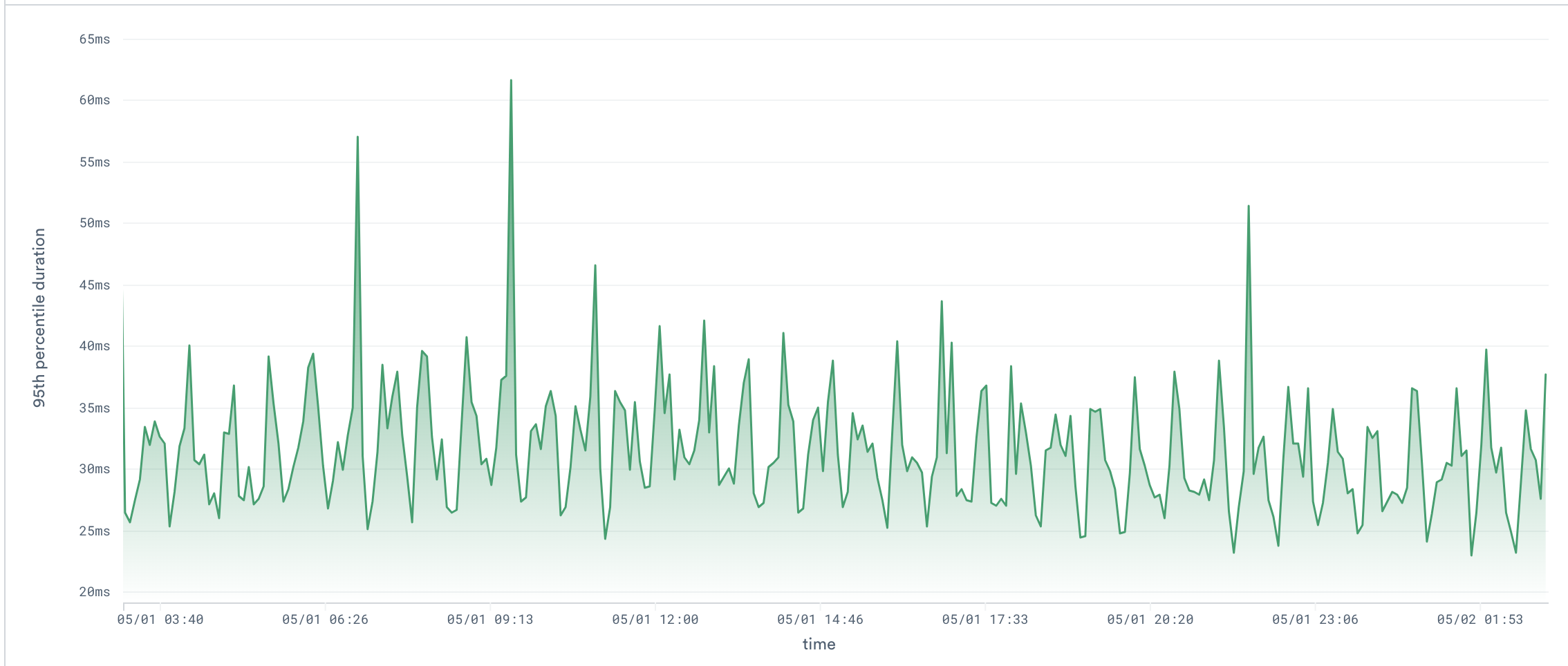
This can be quite slow and expensive to compute, since every single time we want to visualize a different time range, we need to re-aggregate potentially millions of order placement spans.

Observe allows you to pre-aggregate and materialize such data into a downstream dataset, which makes visualizing the chart at different time windows extremely fast and much cheaper.

Let’s see how to leverage the power of Observe and achieve this in OPAL!

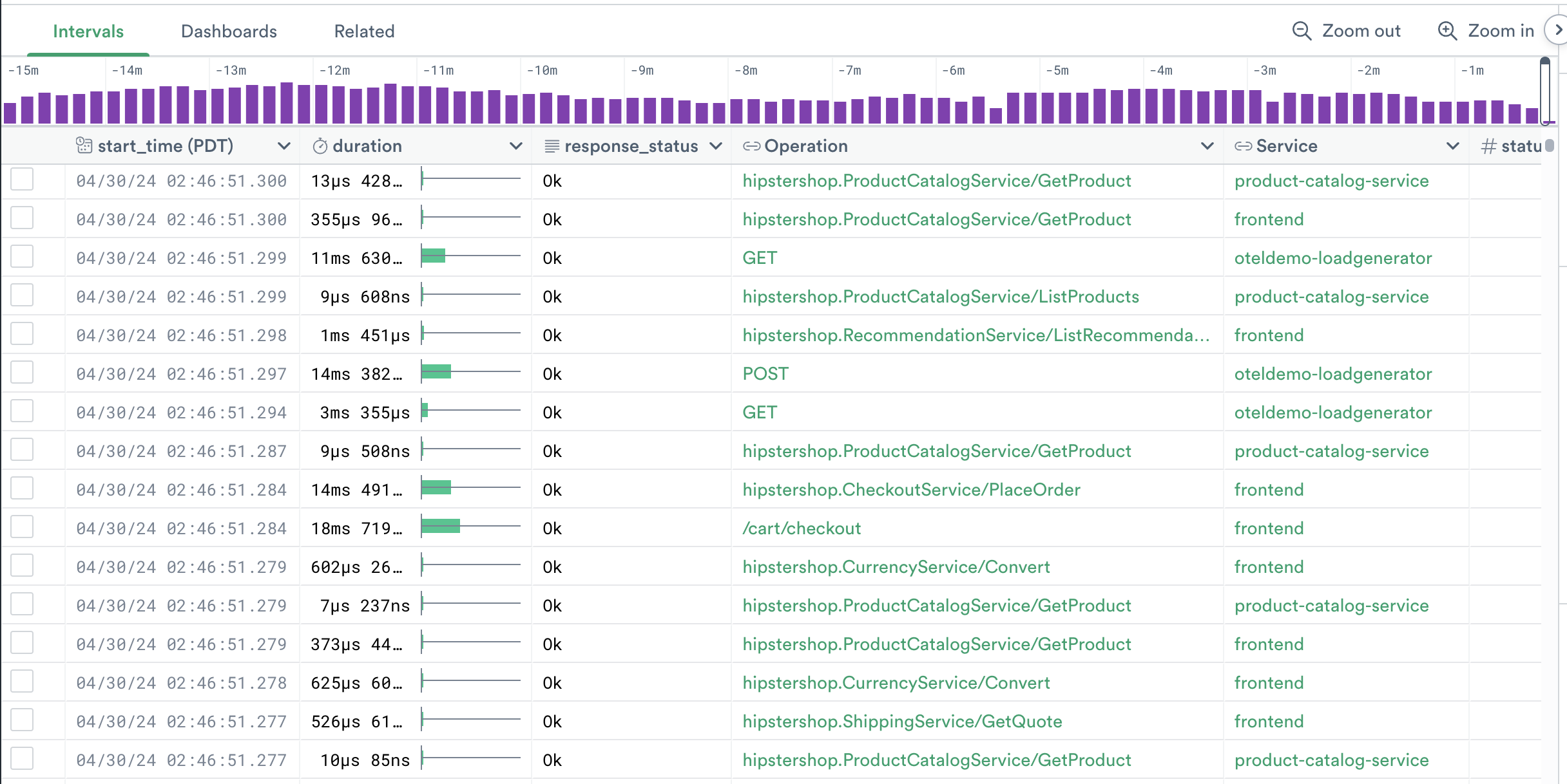
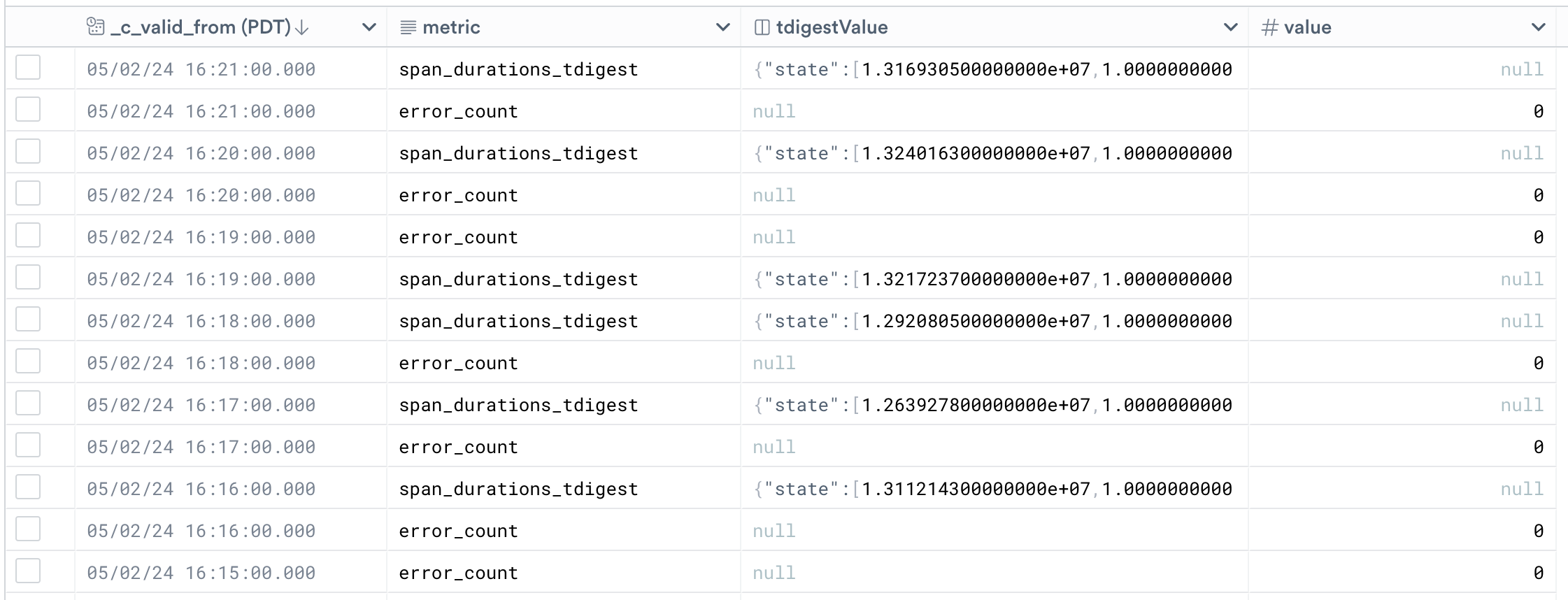
Our starting dataset looks like this:

Firstly, we need to filter out only the Spans we are interested in:

filter service_name = "frontent" and label(^Operation) = "hipstershop.CheckoutService/PlaceOrder"
// Turn Spans into events to make subsequent operations even faster
make_event

Note

This dataset only contains the operation_id, which Observe automatically links to the “Operation” dataset to be able to show you a more meaningful Operation name. To filter by Operation name, we must use the label(^…) syntax to tell Observe to follow the link and use the Operation name, rather than its ID.

make_event is metadata-only and not strictly necessary, but it will improve the performance (and reduce the cost) of the next operations.

Now we must create a metric dataset with the Span durations as metric values. The first step is to turn the events into a time series.

Without tdigest, we could do so with:

timechart 1s, avg_duration:avg(duration), group_by()

The downside of this approach is that we won’t be able to extract a percentile out of multiple data points once they are aggregated into a single duration point in the time series with avg(). This is where tdigest comes to help. It allows us to aggregate numeric data as much as we want into a single tdigest point in the time series, and still be able to extract an accurate (although approximate) percentile out of it afterwards! 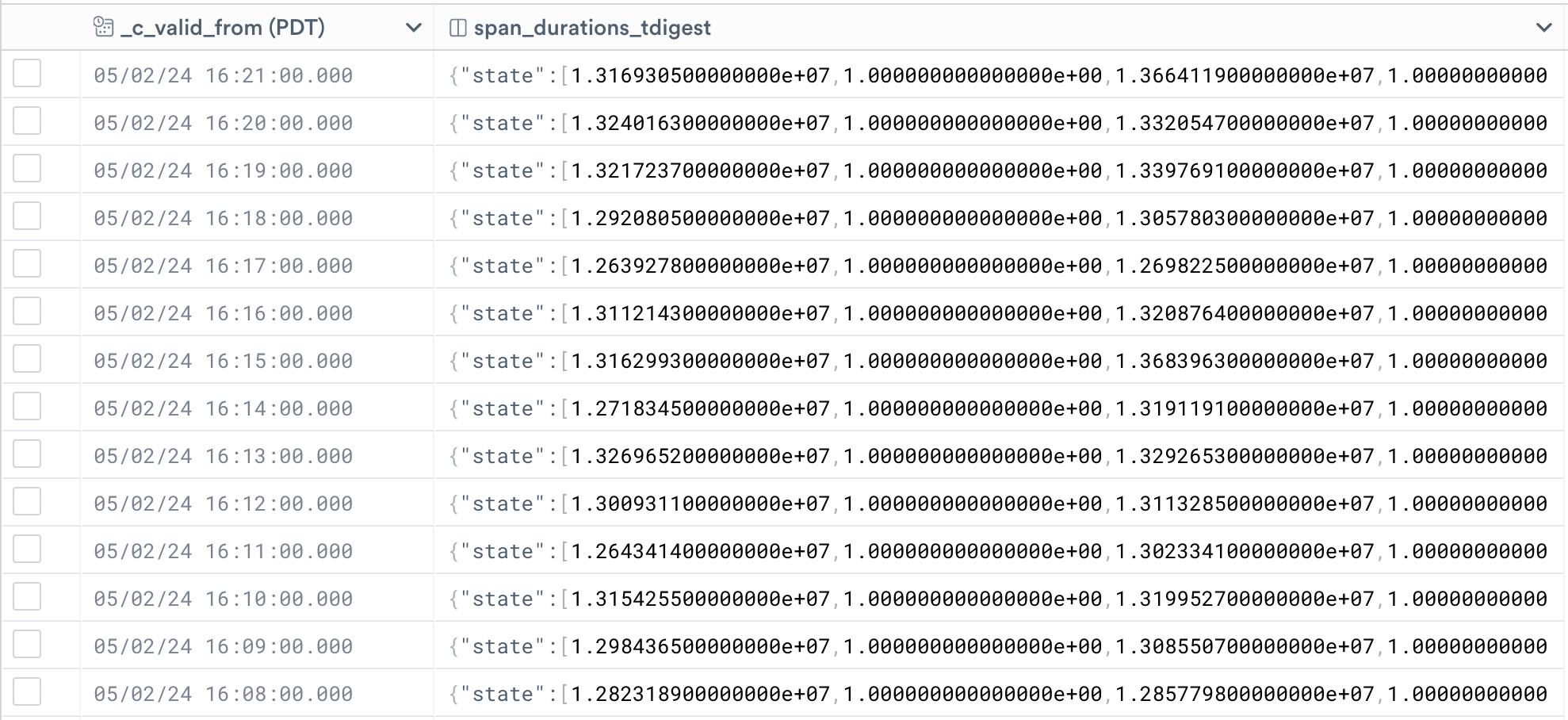Let’s then create a time series with a tdigest value each second:

timechart 1s, span_durations_tdigest:tdigest_agg(duration), group_by()

Note

timechart without group_by() uses the keys as default grouping. Without group_by(), we would have a different time bin per span ID. This is not what we want, as the goal of this step is to combine durations of all spans within a time bin. To override grouping by the default grouping keys, we add group_by() without arguments.

In real use cases, you could group_by() production environments, cluster, or any other differentiatior you might be interested in.

Our dataset now contains time buckets of 1s each, with a tdigest state summarizing all durations of the selected span that happened within the time bucket.

Now we need to give this time series a name and turn the dataset into a metric dataset, to unlock the full power of metrics. There are various ways to do this, the most intuitive way is the following:

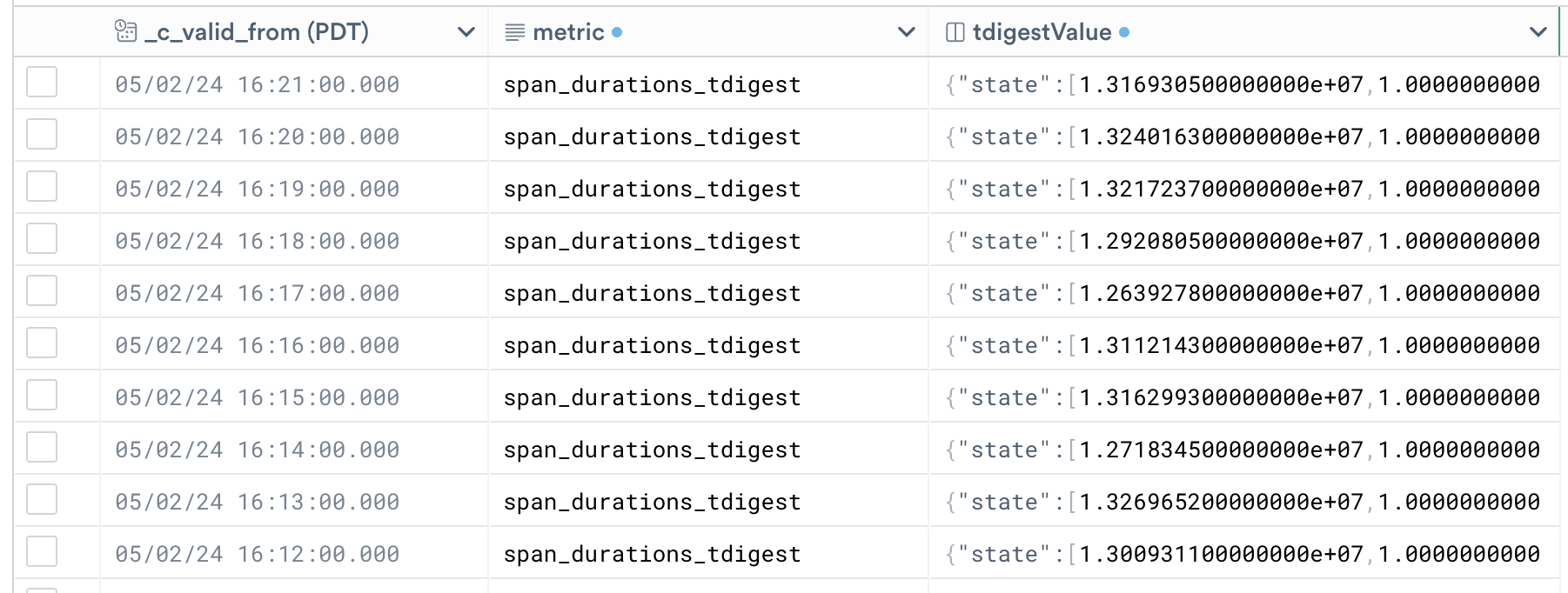
unpivot "metric", "tdigestValue", span_durations_tdigest

We must now adhere to the “metric” interface, which means satisfying the following requirements:

• A “metric” column, containing the metric names –> We already have that

• A float64 “value” column:

  make_col value:float64_null()
  

  We just set all rows to null, since our dataset only contains one tdigest metric and no float64 metrics.

• An optional “tdigestValue” column (in this case it is required, since we have one tdigest metric) –> Also already present

Note

unpivot turns a wide format dataset into a narrow-format one. In particular, it puts all values of one or more columns into a single column called “tdigestValue” (in this case, only values from the “span_durations_tdigest” column), and maintains the information about “which column this value belonged to” into a column called “metric”. The outcome is that the name of the column used in timechart will become the metric name! make_event is once again necessary, since the output of unpivot is of type “interval”, whereas metrics must be events.

We now have a narrow metrics dataset!

Let’s now customize this metric to make sure it appears in the metric explorer for visualisation.

// First apply the metrics interface
interface "metric", tdigestValue:"tdigestValue"

// Set the metric
set_metric options(type:"tdigest"), "span_durations_tdigest"

DONE! The “derived” metric is now registered in Observe and will appear in the Metric Explorer for easy visualization.

The dataset created with this worksheet can now be exported and materialized, to make querying it much faster and cheaper. You can now visualize the order placement latency at any point in time, without having to re-aggregate all the spans!

Creating multiple derived metrics from the same dataset

The process to create more than one metric (of arbitrary types) for the same input data is similar, with a few additions. Firstly, we must add all time series to the same timechart. In this case, let’s add a metric that tracks the spans with an error over time.

timechart 1s, span_durations_tdigest:tdigest_agg(duration), error_count:sum(if(not is_null(error), 1, 0)), group_by()

Let’s then add it to the unpivot statement:

unpivot "metric", "value_variant", span_durations_tdigest, error_count

The “value_variant” column is a variant, and it contains both tdigest and float64 values. Since we want to adhere to the “metric” interface, and given that we have both tdigest and float64 metrics in this dataset, we must have a float64 “value” column and a tdigest “tdigestValue” column. To do so, we can use the following conditional OPAL:

make_col value:if(metric = "error_count", float64(value_variant), float64_null())
make_col tdigestValue:if(metric = "span_durations_tdigest", tdigest(value_variant), tdigest_null())

make_event

This will create a “value” column, which is populated with the (float64) value contained in the “value_variant” column only when the metric is a float64 metric. Otherwise it will contain null. The same applies for the “tdigestValue” column, which will contain the (tdigest) value contained in the “value_variant” column only when the metric is “span_durations_tdigest” (which we know is of type tdigest), otherwise null.

We can then apply the metric interface and call set_metric on all the metrics we just defined the same exact way we did in the previous example.