Collect and use metrics
Types of metrics collected by Observe
Metric type is used to drive default visualization behaviors in metric expression builders (such as Metrics Explorer or a Threshold Metrics Monitor . The metric type also affects the behavior of alignment function that are sensitive to metric types, such as rate and delta .
NoteThe Metric type drives default visualization behavior. If the default is not the desired behavior, you can easily switch the alignment functions in the expression builder: for instance, change
avg()torate()or changerate()todelta().
You can view the type of an ingested metrics dataset by hovering over the name in Metrics Explorer. It is useful to confirm that the type is set correctly, as false positive or negative results could occur from incorrectly typed metrics.
Supported metric types
Observe supports the gauge, cumulativeCounter, delta, and tdigest metric types:
The gauge metric type represents a snapshot of the state at the time of collection. Use a gauge metric type to measure data that is reported continuously, such as available disk space or memory used. The value of a gauge metric can go up or down or stay the same.
Given a series of memory measurements, such as pod_memory_working_set_bytes from Kubernetes, an example data series might look like 31, 30.5, 31, 31, 31.5.
In a gauge metric of pod_memory_working_set_bytes, all reported values are retained. Query time parameters are then used to calculate and display what the user requires.
Set the metric type
The metric type can be explicitly set with set_metric . Whenever the metric type is not explicitly set, Observe will attempt to auto-assign a metric type. This is true for all float64 metrics (gauge, cumulativeCounter and delta). Metrics of type tdigest cannot be automatically discovered by Observe. Use set_metric options(type:"tdigest"), "metric-name" to get the correct metric visualization behavior for tdigest metrics.
Metric types do not affect how metric data is collected or stored, but they are used at query time. A metric is tabulated to make a chart or test a monitored condition. This requires a time resolution, which Observe dynamically determines based on your query window size. For instance, a query window of four hours would have a resolution of one minute; while a query window of one day will have a resolution of five minutes.
The chart or table's behavior is also established by using an OPAL alignment function . This is a mathematical operation used on the values in each time resolution window to determine which value to show in the table or chart. For instance, a metric might have points at every thirty seconds, while our chart has a five minute resolution. This means each five minute window has ten measurements to evaluate. The avg() function will show the average of those ten values.
Metric types affect the run time behavior of some operations that use alignment functions .
delta: calculates the value difference of the argument in each time bin for each group.deltamay produce negative values when the argument decreases over time.- for gauge metrics,
deltaretains the default behavior. Negatives may be produced when the value is decreasing. - for cumulativeCounter metrics,
deltawill assume the values to be monotonically increasing, and treats decreasing values as counter resets. Negatives will not be produced forcumulativeCountertype metrics. - for delta metrics,
deltawill sum up the values in the time window to return the total sum. Negatives may be produced for negative input values.
- for gauge metrics,
delta_monotonic: calculates the amount of difference in a column in each time bin for each group.delta_monotonicby default assumes the argument to be monotonically increasing, and treats decreasing values as counter resets.- for gauge and cumulativeCounter metrics,
delta_monotonicretains the default behavior of assuming monotonic increases. - for delta metrics,
delta_monotonicwill sum up the values in the time window to return the total sum. Negatives may be produced for negative input values.
- for gauge and cumulativeCounter metrics,
deriv: calculates the average per-second derivative of the metric during each time frame- for gauge metrics,
derivcomputes the value change over the time frame, allowing negative changes, and then divides the value change with time frame size. - for cumulativeCounter metrics,
derivcomputes the value change over the time frame, treating value decreases as counter resets to prevent negative changes, and then divides it by the time frame size. - for delta metrics,
derivcomputes the value change by summing up the deltas, and then divides it by the time frame size.
- for gauge metrics,
rate: calculates the average per-second rate of increase of the metric during each time frame- for gauge and cumulativeCounter metrics,
ratecomputes the value increase over the time frame, assuming monotonic increase in the value and treating decreasing values as counter resets, and then divides the value increase by the time frame size. - for delta metrics,
ratecomputes the value increase by sums of the deltas, and then divides it by the time frame size.
- for gauge and cumulativeCounter metrics,
Understand aggregation
Aggregation is a computation that rearranges a time series into regular time intervals, aggregating multiple data points of a time series into one data point for each time interval.
Aggregation along the time dimension (alignment)
Metrics are usually very dense (contain lots of measurements at a high frequency). It is often useful to visualize a metric over time at more user friendly intervals. For example, disk usage metrics might have one value every 5 seconds, and we might want to plot such usage over the Black Friday week. Therefore, the ideal plotting format would be to have disk usage summaries every 10 minutes.
A typical alignment operation looks like this:
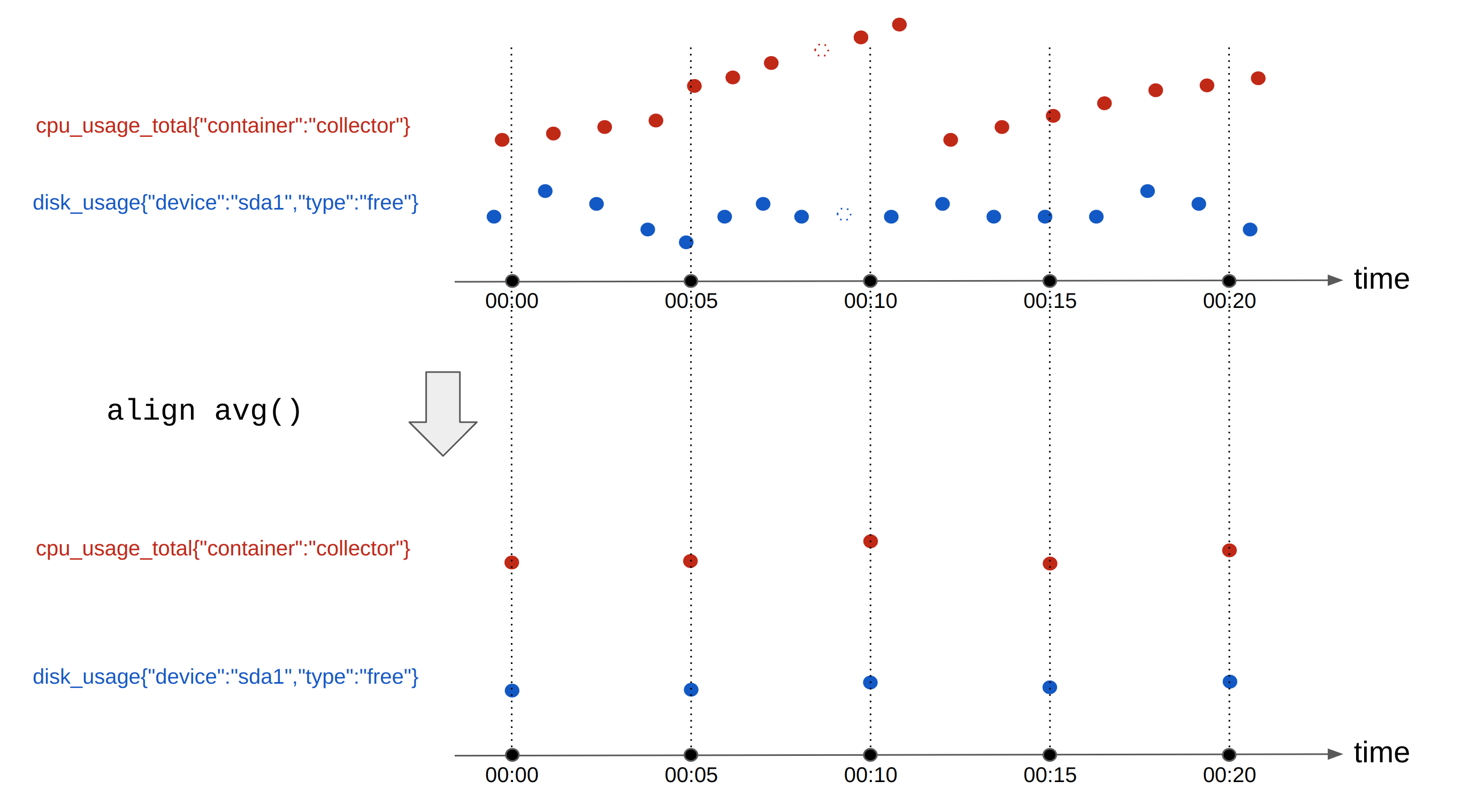
You can see that each cpu_usage_total point is not exactly vertically aligned with each disk_usage point. Before we can aggregate the data, we take the three red points between 00:00 and 00:05 and average them on the 00:05 line, then take the four blue points between 00:00 and 00:05 and average them on the 00:05 line. This is repeated for each interval, so we now have alignment on the average values.
In addition to using avg() for alignment, you can also use other functions, such as the following:
- Use
last()to mimick the default behavior for Prometheus. This function uses just the last point in each interval for alignment, and drops the other values. - Use
max()to take only the largest or highest value in each interval for alignment. - Use
min()to take only the smallest or least value in each interval for alignment. - For cumulative counter metrics, use
rate()orderiv()to view the rate over time, such as the number of requests per second, anddelta_monotonic()ordelta()to view the absolute change in value between the first point and last point, regardless of time.
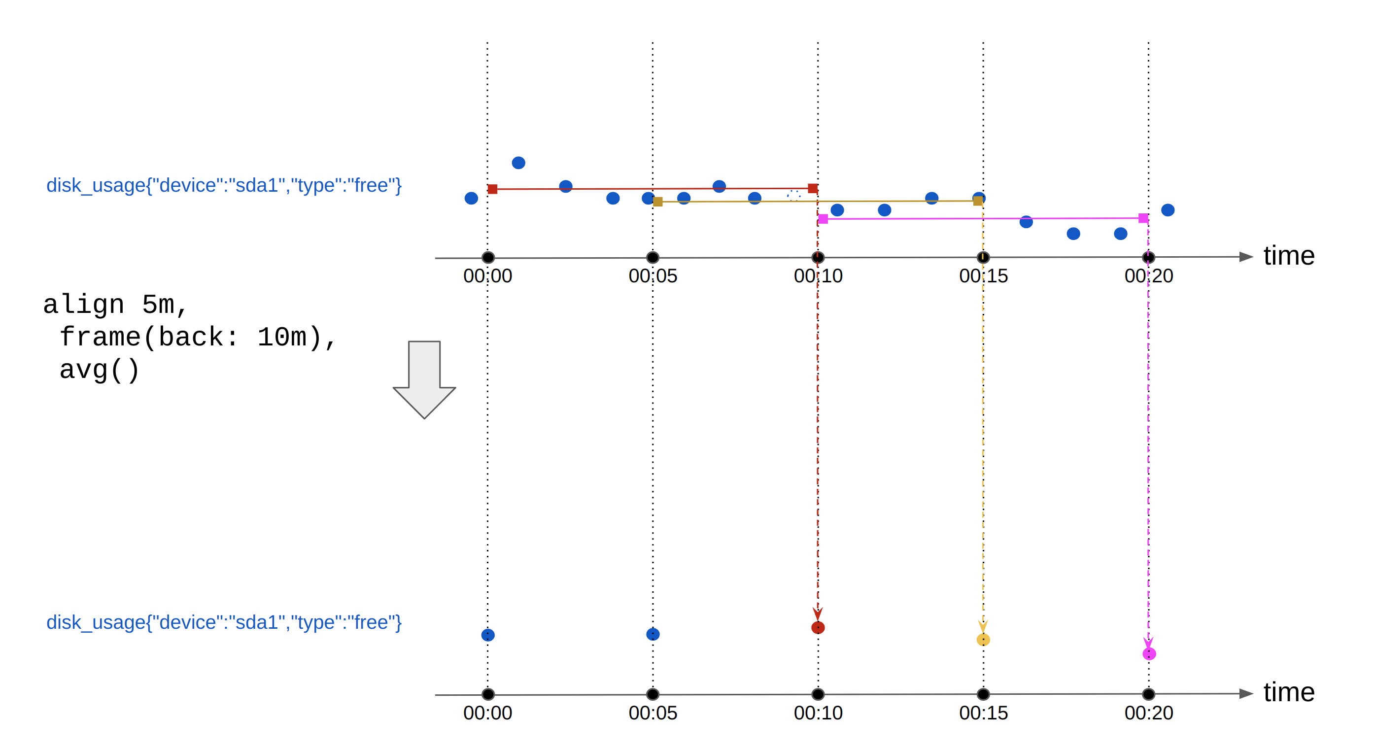
A more advanced version of alignment is sliding window alignment, also known as hopping window alignment. It is used for computations like “rolling average”. In this query, for each time-series, we generate one output point every 5 minutes, by computing the average of the input points in the prior 10 minutes. For example:
Aggregation along other dimensions
Time series can be aggregated across tags. For instance, consider the same metric disk_usage being reported for different usage types, such as free or used. You can add them up to get the total disk space.
To accomplish this, use a tag-dimension aggregation operation that aggregates multiple (already aligned) time series into one. Tag-dimension aggregation takes in regularly aligned time series, and keeps the timestamps unchanged. Aggregation across tags also requires an aggregation function to be specified.
Conceptually, tag-dimension aggregation looks like this:

Additional metrics metadata
In addition to the metric type, the following metadata items can be set:
- Measurement type - describes the type of data reported in each data point. Observe supports
float64andtdigestas metric data types. - Unit - describes the unit of measurement such as
kborkB/s. - Description - detailed information about the metric.
- Tags - For a time series, tags better describe and differentiate the measurements. You can use them to identify individual times series during metric computations such as
alignandaggregate.
A Metrics Dataset contains metric data recognized by Observe. Observe optimizes the metric dataset for scalable ingestion and queries, supporting a large number of metrics. A metric dataset has the following properties:
- Each row in the dataset table describes one point in a time series.
- A metric dataset contains a
stringtype metric value column namedmetric. - Contains a
float64metric value column namedvalue. - Contains a
valid_fromcolumn with the measurement time for each data point. - The
metricinterface OPAL language designates a dataset as a metric dataset. - All non-metric names, values, and non-valid_from columns contain metric tags.
A Metrics Dataset is always an Event Dataset and the data either inherited from an upstream Metrics Dataset or created using the OPAL interface verb. Metrics use OPAL in a worksheet to transform the raw data, add metadata, and create relationships between datasets. If you are not familiar with OPAL, please see What is OPAL?
A metric dataset contains one metric point per row - a single data point containing a timestamp, name, value, and zero or more tags. For example, the following table contains values for two metrics:
| valid_from | metric | value | tags |
|---|---|---|---|
| 00:00:00 | disk_used_bytes | 20000000 | {"device":"sda1"} |
| 00:00:00 | disk_total_bytes | 50000000 | {"device":"sda1"} |
| 00:01:00 | disk_used_bytes | 10000000 | {"device":"sda1"} |
| 00:01:00 | disk_total_bytes | 50000000 | {"device":"sda1"} |
| 00:02:00 | disk_used_bytes | 40000000 | {"device":"sda1"} |
| 00:02:00 | disk_total_bytes | 50000000 | {"device":"sda1"} |
Some systems generate this by default, or you can shape other data into the correct form with OPAL.
Metric values must be either float64 or tdigest. If you need to convert numeric types to float64 see the float64 function. To create tdigest objects, use the tdigest_agg function. To combine tdigest states in any dimension, use the tdigest_combine function.
| input | function | output |
|---|---|---|
| single numeric values | float64 | float64 numeric values |
| array of numeric or duration values | tdigest_agg | tdigest JSON object |
multiple tdigest objects | tdigest_combine | tdigest JSON object |
| input | function | output |
|---|---|---|
| single numeric values | float64 | float64 numeric values |
| array of numeric or duration values | tdigest_agg | tdigest JSON object |
multiple tdigest objects | tdigest_combine | tdigest JSON object |
tdigest metrics behave in a slightly different way. Since their value cannot be stored in the same column as other metrics' values (because the value type is not float64), metrics datasets are allowed to have a second value column to store tdigest metrics' values and might look like this:
| valid_from | metric | value | tdigestValue | tags |
|---|---|---|---|---|
| 00:00:00 | disk_used_bytes | 20000000 | null | {"device":"sda1"} |
| 00:00:00 | disk_downtime_nanoseconds | null | {"type":"tdigest","state":[15,1],"version":1} | {"device":"sda1"} |
| 00:01:00 | disk_used_bytes | 10000000 | null | {"device":"sda1"} |
| 00:01:00 | disk_downtime_nanoseconds | null | {"type":"tdigest","state":[15,1,30,1,2,1],"version":1} | {"device":"sda1"} |
| 00:02:00 | disk_used_bytes | 40000000 | null | {"device":"sda1"} |
| 00:02:00 | disk_downtime_nanoseconds | null | {"type":"tdigest","state":[],"version":1} | {"device":"sda1"} |
Note that each metric point must have either the value column or the tdigestValue column populated. The other column should be null. This is because each row in the metric dataset corresponds to one point in one time series. Points that belong to time series "disk_downtime_nanoseconds" (a metric of type tdigest) should only contain tdigest values.
Updated 4 months ago