What is OPAL?
The Observe temporal relational model considers time, and tracking system data over time, an integral part of data modeling. Yet traditional attempts to model the time-varying nature of data on top of relational databases have ended up with non-standard SQL extensions. These mechanisms can be fragile and hard to use.
The Observe platform solves this problem by providing a language for expressing the kinds of operations you want to perform as a user of the system and takes care of the time-dependent factors.
And since every UI action generates an OPAL equivalent, writing code by hand instead of using the UI doesn't replace the UI. You may choose to perform some operations in the UI, some in code, and some by starting with the UI and expanding in code.
Get started
We recommend starting with Anatomy of an OPAL pipeline and OPAL Data types and operators to understand the basics. Then begin exploring your data in a Worksheet. Read OPAL syntax for more about the structure of OPAL statements.
Want to get hands-on? Go to the Get started with OPAL tutorial.
Other helpful topics:
- See OPAL syntax to learn how to write OPAL statements and pipelines.
- See OPAL performance cookbook for best practices when writing queries and data modeling.
- See OPAL examples for some examples of common OPAL operations.
- See OPAL verbs for the OPAL verb reference.
- See OPAL functions for the OPAL function reference.
Anatomy of an OPAL pipeline
An OPAL pipeline consists of a sequence of statements where the output of one statement is the input for the next. This could be a single line with one statement or many lines of complex shaping and filtering.
A pipeline contains four types of elements:
- Inputs - define the applicable datasets.
- Verbs - define what processing to perform with those datasets.
- Functions - define transforming individual values in the data.
- Outputs - pass a dataset on to the next verb or the final result.
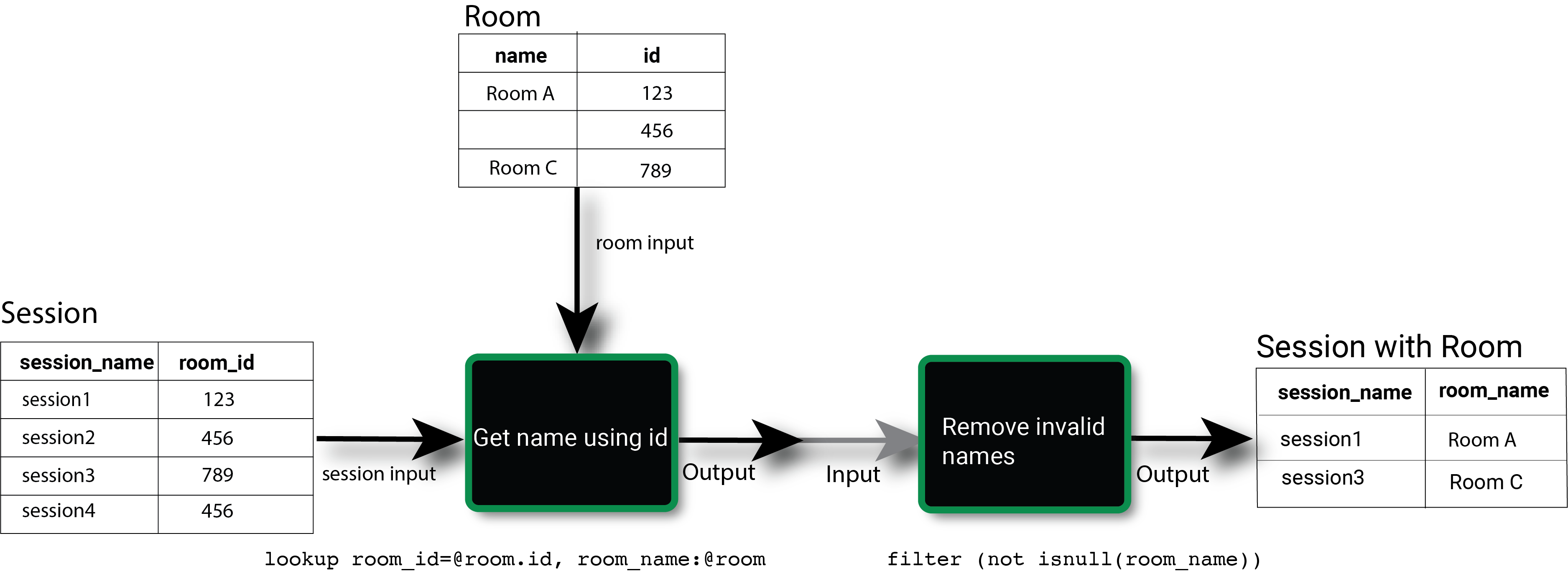
A complete pipeline, also called an OPAL script, consists of a series of inputs, verbs, functions, and outputs that define the desired result. The following diagram illustrates combining multiple elements together as the first verb statement passes the results of the lookup operation to a second verb, which uses a function to remove null values.
Inputs
Pipeline inputs consist of datasets, such as an Event Stream. Pipelines may use as many datasets as required, although individual verbs vary in the number of accepted datasets. For example, lookup accepts a main input dataset containing the field of interest and a lookup table dataset that maps those values to more useful ones.
A pipeline might be a single sequence of steps from input to output, or it may contain subqueries with individual processing of particular inputs. You can combine both for more complex operations. (See OPAL syntax for more details.)
Verbs
Verbs make up the main actors in a pipeline. Each takes a primary input, either the initial dataset or the output of the verb before it goes into the pipeline. Some verbs accept multiple dataset inputs, such as a join operation. A verb outputs exactly one output dataset.
TipSee the OPAL verbs for details on individual verbs.
The most important verb is filter, which takes the default input and returns data matching the condition defined in the filter expression. This is analogous to the WHERE clause in a SQL query.
OPAL verbs and accelerated datasets
An important consideration is if the verb you use allows the resulting Dataset to be accelerated. Most Observe Datasets are really Datastreams. New data is always being added, but any particular operation may be interested in only some of it.
OPAL considers most verbs to be streaming operators since they transform one or more input data streams to an output data stream, and only then identify which results within the desired query time window.
When you apply filter to an input, OPAL applies the filtering condition check to each event. All events that pass the check form an output dataset. filter then queries the results, essentially selecting the desired set of events. The data does not change.
This works because filter functions the same way for any size query time window. Any individual observation is either included in the results or not, without considering the disposition of neighboring observations. Observe refers to this as "capable of being accelerated." As long as all the verbs in an OPAL pipeline allow acceleration of the results, the output dataset automatically accelerates to provide better query performance.
However, a few verbs cannot be accelerated. This means the output is different for different size query time windows, and the original filter must be applied each time you query the dataset.
These verbs still perform many useful functions, particularly for ad hoc analysis in a Worksheet. But you can't create a new dataset from those Worksheet results, as it can't be accelerated. To create a new dataset from a Worksheet, ensure that all of the OPAL can be accelerated before you publish a new event Data stream.
Types of verbs
OPAL organizes verbs into several categories, based on the action they perform. Some verbs have more than one category.
| Verb category | Description |
|---|---|
| Aggregate | Aggregate verbs work with aggregate functions to summarize data. |
| Filter | Filter verbs select events matching an expression or condition, similar to SQL SELECT WHERE. A filter statement might match a pattern, literal or regular expression, or return the top values for a group of values. |
| Join | Join verbs combine data from multiple datasets to generate an output value. For example, a union operation adds new merged and appended fields from other event datasets to the primary input dataset. The flatten family of verbs is also included in the Join category, as a special case of joining a dataset with itself to create new output events. |
| Metadata | Metadata verbs add information about the dataset, rather than act on the data it contains. These verbs add additional context about the dataset contents or define relationships between datasets. Common metadata operations consist of configuring foreign keys, registering types of metrics, and creating resources from event streams. |
| Metrics | Metrics verbs specify how metrics are defined and aggregated, such as specifying the units of reported values. |
| Projection | Projection verbs create or remove fields based on existing fields or values. For example, pick_col selects only the desired fields, dropping all others. |
For the complete list of verbs by category, see OPAL verbs.
Functions
Functions act on individual values rather than datasets. Where verbs are set operations, acting upon inputs sets and returning output sets, a function is a scalar operation. It returns a single value.
TipSee the OPAL functions for details on individual functions.
Types of functions
OPAL features the following general types of functions:
- Plain, or scalar functions
- Summarizing, or aggregate functions
- Window functions
Plain or scalar functions
These functions act on values from an input event field, such as converting a timestamp or comparing two values. Scalar functions always output a single value per input event.
Example: replace_regex()
make_col foo:"foo4-bar2" // input text
make_col bar:regex_replace(foo, /^([A-Za-z]{3})([0-9]{1})-([A-Za-z]{3})([0-9]{1})$/,'\\3\\2-\\1\\4', 0)
// result: new column bar containing "bar4-foo2"
Summarizing, or aggregate functions
Within an aggregating verb statement (such as statsby), calculate a summary of multiple values across multiple input events. For example, avg() calculates the average of a field's values across all input events that match the statsby group_by field. This is similar to GROUP BY in a SQL query. Aggregate functions typically output fewer events than are in the input.
Example: count() with verb statsby
statsby "reportsPerSensor":count(sensor), group_by(sensor)For a list of all aggregate functions, see OPAL aggregate functions.
Window functions
Within a window() statement, a window function looks at the input events in the window and calculates an output value for each input event. For example, avg(), when applied to a window, calculates a moving average for a fixed window size over time. window() and window functions are used with make_col and similar verbs, where the window() statement is an argument defining the contents of the output column.
Example: first()
// get name of the earliest sensor to report in the current window
make_col FirstToReportData:window(first(sensor))
For a list of all window functions, see Window Functions.
Generally, functions take expressions as arguments, and can themselves be part of an expression. max(num_hosts+3) is just as valid as max(num_hosts)+3.
Scalar functions may be used anywhere an expression can be used. Use aggregate and window functions with aggregating verbs to perform more complex operations. Some functions may be either aggregating or windowing, depending on the verb used with them.
Functions also have a category, to aid in locating the correct function to perform your desired operation. For more, see OPAL functions.
Output
The results of a pipeline may be presented in a variety of ways. It could be statistics like top K values, histograms, or small line charts (sparklines) for each column in the output dataset. When you query or model in Observe, OPAL handles many of these details for you. With OPAL pipelines, you control how to display your output.
Use O11y Copilot with OPAL
o11y AI uses artificial intelligence (AI) to offer auto-completion as you write OPAL queries. You can receive suggestions from the o11y AI either by starting to write the OPAL you want to use, or by writing a natural language comment describing what you want the code to do. o11y AI analyzes the context in the file, as well as related files, and offers suggestions from within the OPAL console.
For example, if you follow the instructions in the Model weather data tutorial, and you activate o11y AI using cmd + K on a Mac or Ctrl + K on a PC, you may see suggestions similar to the following:
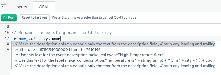
Use o11y AI any time you need assistance with the OPAL language.
Updated 6 months ago