Advanced Observe Concepts¶

Data Acceleration¶

Observe performs dataset acceleration using background processes, which periodically and incrementally compute and update the dataset state. Observe materializes a dataset state by processing any changes to the input consisting of newly arrived events.

An OPAL pipeline for a dataset consists of a hierarchic application of OPAL commands from the source observation datasets to the eventual dataset. A dataset is accelerable if the fully expanded definition, or OPAL pipeline, can be accelerable.

Any query can be published into a dataset, reused, and queried for different query windows. Datasets can also be published on top of other datasets, forming a pipeline.

Note

You can accelerate the dataset for the full queried time range to speed up future queries. However, this operation does consume Observe credits.

Learn more about data acceleration in About Queries and On-demand Acceleration.

Time Dilation¶

Each query in Observe has a query window, also called the output window of the query. It means “compute all results that fall into this time range” rather than “read the input data that falls into this time range”.

The distinction doesn’t matter for simple queries such as a single filter over an event stream. But it can make a significant difference for more complex queries.

For example, suppose you want to compute the daily sum of system error counts using the following query:

time_chart 1d, sum(system_error_count), group_by(server)

If you want to review a query window for the last four hours, compute the correct result, then sum over a one-day bucket, you must look at more than four hours of data. The timechart verb needs to dilate the input time window of the query to a full day that covers the query window. This means a six-fold or twelve-fold increase in the input data volume compared to the undilated query window.

The following is a list of common OPAL verbs that can incur time dilation:

make_resource - dilation amount determined by the expiry setting of the verb.
time_chart - dilation amount determined by the bucket size
window functions - dilation amount determined by the window frame
set_valid_from - dilation amount determined by the max_time_diff option.

Time dilation can be a significant cost driver for transforms, which may need to read overlapping input data for successive executions repeatedly.

Acceleration Window¶

Observe calls the time range for which a dataset has materialized the acceleration window of the dataset. Queries whose input datasets have been accelerated for the query (dilated) input window are much faster than queries on the raw input data loaded into Observe initially.

Non-accelerable datasets are always inlined when queried. Examples of datasets with non-accelerable OPAL include the following:

Nondeterministic functions such as query_start_time()
Verbs used without an explicit frame, such as these:
- ever, never, exists, follow
Combinations of verbs, functions, and options:
- timechart options(empty_bins:true)

Input Data Volume¶

Queries can require different amounts of input data volume. The product of the following factors can determine input data volume:

Read window size - the size of the time range that the query needs to read.
Input data rate - the number of rows per second or bytes per second arriving in the input datasets.
Input columns - which columns in the input datasets need to be read.

Observe uses a column-oriented data layout. Queries only need to read the columns used. This saves time and credits.

For example, if a query reads 10 hours of data from an event dataset with 1,000,000 events per hour, the query reads approximately 10,000,000 rows. The exact quantity of bytes read depends on the set of input columns and the compression factor of these columns, which can range from a few bytes per row to hundreds of kilobytes per row.

Inline Queries¶

Immediately after you define a new dataset, Observe has not yet been able to materialize the state and accelerate it. Observe can temporarily inline the dataset to allow users to use the dataset immediately. Inlining means Observe computes the dataset on the fly by inline-expanding its OPAL definition and prepending that OPAL to the main query.

The same inlining happens when users query historic time ranges that fall outside the dataset’s acceleration window. Such inlining makes the query more complex, potentially reads more input data, and likely to consume additional credits.

Observe never performs more than one level of inlining and does not support nested and recursive inlining. This is to prevent excessive query latency and high costs.

A dataset can be one of two types:

A source dataset associated with a Datastream
An OPAL pipeline defined on top of other datasets

When Observe queries a non-source dataset, one of two actions occurs:

If the dataset is accelerated, the query reads the materialized table.
If it is not, the OPAL definition is inline expanded and prepended to the query.

Query Size¶

Observe attempts to select the ideal data warehouse size to run a given query. Therefore, Observe needs to estimate the size of the query and bases the size of a database query on two factors:

Query complexity - the amount of work required per byte of input data
Amount of input data - the quantity of data in bytes

Besides execution time driven by these two factors, the overall query execution time also depends on these additional three parameters:

Query compilation time - translating OPAL into the optimal execution plan
Initialization overhead, such as spawning processes or opening network connections
Returning query results

For queries with very little input data, the time spent on these other factors can exceed the actual execution time spent on processing data.

Query Complexity¶

An Observe query consists of a pipeline of OPAL verbs and functions. Some verbs are more expensive than others because they perform more work per input row. For example, the lookup verb needs to find all matching pairs of rows of two input datasets according to a link established between the two datasets. It needs to find all pairs of rows with matching key fields and overlapping time intervals.

Verbs used with joins such as lookup, ‘join’, and follow, as well as aggregations such as time_chart, and make_session require more processing time than simple verbs such as filter and make_col.

Transform Queries¶

Observe performs dataset acceleration using background queries called transforms. Transform queries periodically compute and update datasets incrementally, a process known as “materialization.” Dataset acceleration makes subsequent interactive queries fast and cheap. It is essential for low query cost.

Of course, transform queries also consume resources. It is not unusual to see more Observe credits spent on transforms than interactive queries. However, these costs are necessary; otherwise, interactive queries would be much more expensive and prohibitively slow without dataset acceleration. So these transform credits are typically well spent.

The following parameters determine the cost of executing an individual transform query:

Transform query complexity - the amount of work per byte of data
Input data volume
Output data volume

Observe executes transform queries periodically as new data arrives. Four factors determine the frequency and cost of the periodic executions:

Freshness goal of the output dataset
Acceleration window - time range receiving acceleration
Read amplification - frequency of reading the same input data
Write amplification - frequency of writing the same output data

Each dataset has a configurable freshness goal. If you set the freshness goal to five minutes, Observe materializes the dataset every five minutes. In other words, the delay between receiving an observation and seeing the effect on queries and monitors should not exceed five minutes.

The acceleration window contains a range of time that data materializes. A larger window requires more work and storage overhead.

Read and write amplifications result from time dilation. As an extreme example, a transform may run every hour but contain a time dilation of 24 hours. For every hour, this transform needs to read up to 24 hours of input data and over-write up to 24 hours of output data. The read-and-write amplification of this transform is 24x.

To reduce the credit cost impact of read and write amplification, study the OPAL language documentation and choose the appropriate options for verbs that cause time dilation, such as make_resource, time_chart, set_valid_from, etc.

Monitors are materialized datasets as well, with their own freshness goals and acceleration windows. You can review their freshness goal settings in the Acceleration Manager, by filtering to Monitors.

Freshness Goal¶

The Freshness Goal of a Dataset determines how often Observe runs transform queries to update the dataset in the background and keep the materialized state up-to-date. This Freshness Goal is not a strict upper bound, especially when considering other factors such as cost tradeoffs, freshness decay, and the Acceleration Credit Manager. The Freshness Goal defines the periodical nature of executing transform tasks, and data may be stale beyond the Freshness Goal setting while the Transform task runs in the background. Furthermore, besides the configured Freshness Goal of the Dataset, the usage, as well as the Freshness Goal of downstream Datasets, affects how often Transform queries run.

A Dataset with a more stringent Freshness Goal can consume more Observe credits on accelerations than a dataset with a more relaxed Freshness Goal. Observe runs the Acceleration tasks of Datasets with a more stringent freshness more often and in smaller batches. This effect may be multiplied by read amplification and write amplification caused by time dilation.

The Freshness Goal of a Dataset also affects the cost of upstream Dataset acceleration, as Observe runs the upstream transforms more frequently to satisfy the downstream Dataset Freshness Goal. The minimum of the decayed Dataset Freshness Goals and any downstream decayed Freshness Goals dictates the acceleration execution frequency.

Lowering the freshness goal of AWS RDS Logs may transitively lower the freshness goals of all the upstream datasets in a lineage graph.

Finally, if you enable the Acceleration Credit Manager feature, Freshness Goals may be increased to reduce costs. For more information, please consult the Acceleration Credit Manager documentation.

Freshness Decay¶

Observe has an important cost-saving feature called Freshness Decay. Whenever a Dataset isn’t queried for a while the Freshness Goal is slowly increased to 1 hour. This feature is instrumental in saving Transform Credits as the frequency of Transform Queries is one of the main drivers of their cost (see above).

When a Freshness Goal has decayed beyond the configured goal and a Dataset is queried, the Freshness Goal is immediately reset to the original value. If necessary, that triggers a catch-up transform. As a result, the very first query on a decayed Dataset may see data that can be up to one hour stale. But subsequent queries will see new data again as soon as the Transform Queries have finished.

Figure 8 - Freshness Decay

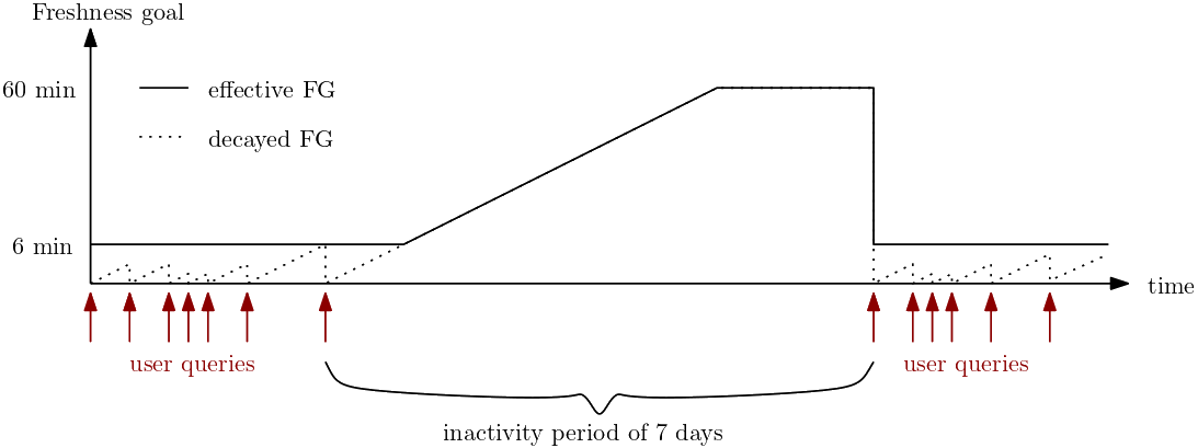
In Figure 8 an example is depicted where the Freshness Goal (solid line) changes in response to the absence of queries by users. The Freshness Goal, which is configured to be 6 minutes, decays at a rate of 1 minute per hour without users accessing it. The decay process stats at a Freshness Goal of 0, such that the Freshness Goal is not affected for the first 6 hours after the last user query. After this, the effective Freshness Goal exceeds the original Freshness Goal. The decay process is shown as the dotted line. Once an effective Freshness Goal of 60 minutes is reached, the goal isn’t increased anymore, as further cost savings are generally small at this point. As soon as the Dataset is queried again, the Freshness Goal and the Transform Queries are executed every 6 minutes.