Basic statements, expressions, and queries

OPAL verbs and functions may be combined to perform more complex operations. For example, create a new field with a constructed string value by using make_col and concat_strings() together:

// New column "location" containing string with both city and country
make_col location:concat_strings(city, ",", country)

Or calculate a value:

// Convert degrees C to degrees F
make_col temperature_f:(temp*9/5 + 32)

Each line (step) of an OPAL script builds on previous ones, so the city example might look like this:

make_col location:concat_strings(city, ",", country)
filter location="Boston, US"

Numeric literals may be decimal, hex, or octal:

make_col octal:int64(0123) // octal 123 decimal 83
make_col decimal:int64(123)
make_col hex:int64(0x123) // hex 123 decimal 291

Subqueries

A standard OPAL query is a linear series of steps with one or more dataset inputs. Each action contributes to the final output, but the data coming from those inputs can't be modified in the process.

Subqueries provide more flexibility, as they allow each input to have unique shaping or other pre-processing. Subqueries dramatically reduce the need for intermediate datasets in complex shaping.

The first subquery in a query may filter a dataset one way, the second another, and a third combine those two results with an entirely different dataset and more actions. Together they produce a result, which might be the final result of your OPAL script or passed as input for additional shaping. Subqueries must be defined before you can reference them but otherwise may be located anywhere in an OPAL script.

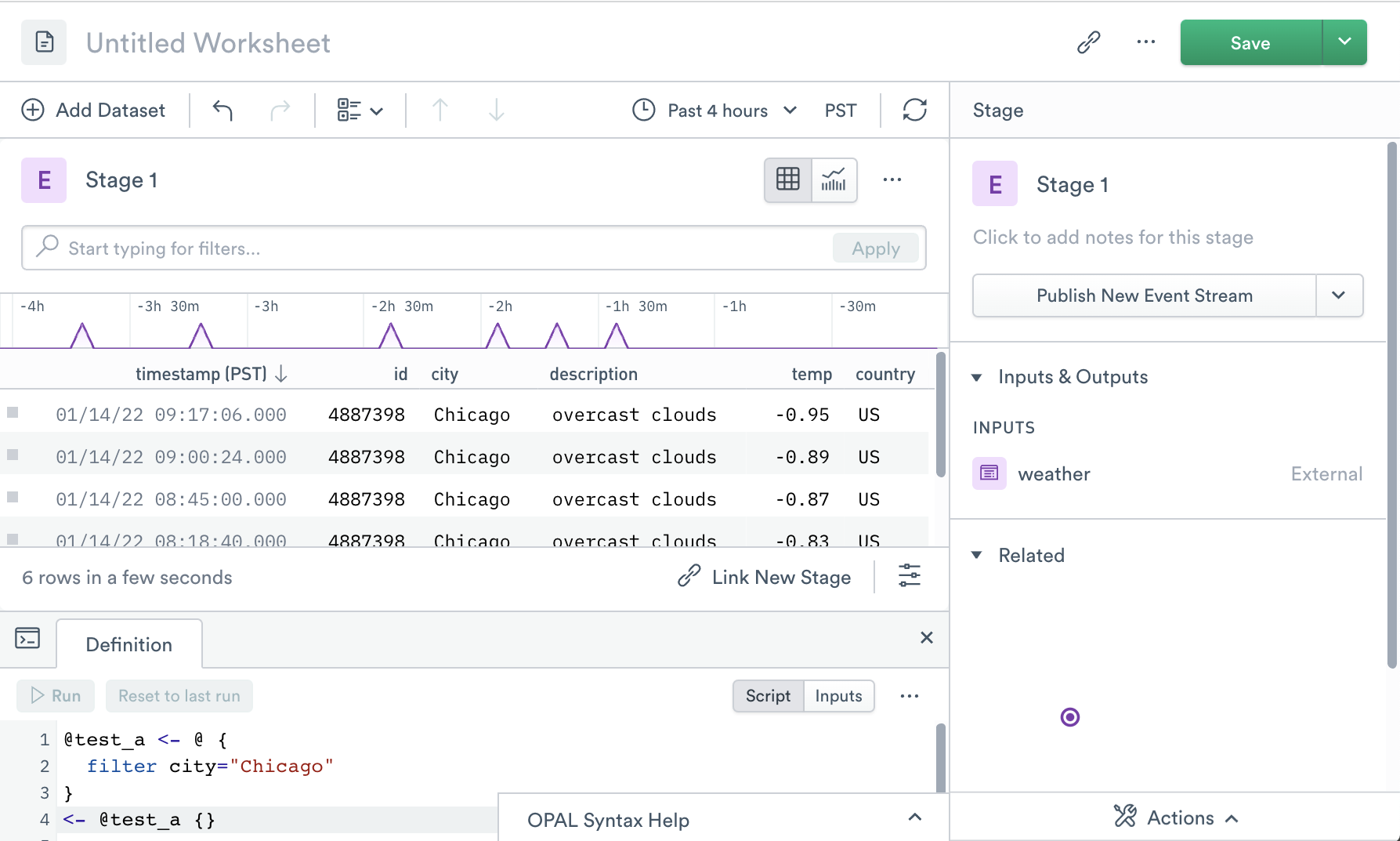
Subquery containing a single filter

The simplest subquery has one definition block and one result block. OPAL does not require a subquery for a basic filter of course, but here it stands in for whatever OPAL your task may require.

In this example, <- @ indicates we are using the default primary input, weather, without explicitly specifying it by name. The final <- @test_a {} invokes @test_a to generate the result.

// Starting from the "weather" dataset, which contains the field "city"
@test_a <- @ {
  filter city="Chicago"
}

// this is the final result of the entire query,
// with subquery @test_a as its input
<- @test_a {}

Either of these blocks may have empty bodies, although without filter city="Chicago" the @test_a subquery would have no effect.

The following example shows a new Worksheet with temperature data for Chicago:

You can also explicitly specify the primary input dataset by name:

@test_a <- @weather {
  filter city="Chicago"
}

For the primary input, you may use either method. Because this is the dataset you originally started with in your Worksheet, Observe can determine what the input dataset should be. Any additional linked datasets, however, must be referenced by name. (See below for examples.)

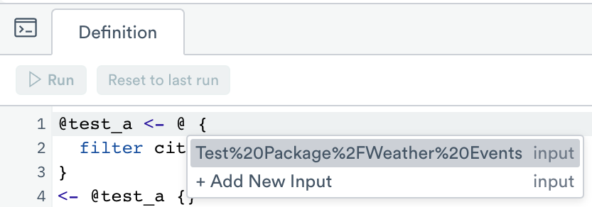
Spaces and other special characters in dataset names must be HTML escaped (example: %2F for /.) You may find it more convenient to select a dataset from the input menu instead:

Subquery results may also be used as input for any verb that accepts a dataset:

// Filter Countries resources to North America
// Resulting @NACountries is now available to use elsewhere
@NACountries <- @Countries {
	filter country = "US" or country = "MX" or country = "CA"
}

// Join (inner join) the subquery results with primary input City
// to get the data for just countries in North America
join country=@NACountries.country
}

Queries containing multiple subqueries

Chain multiple subqueries together by using the output of the first as the input to the second:

// Subquery a
@test_a <- @ {
  filter city="Chicago"
}

// Subquery b
@test_b <- @test_a {
  filter contains(description, "cloud")
}

// Final result only needs the output from @test_b,
// since that builds on previous operations done in @test_a
<- @test_b {}
}

Two subqueries with different operations on the primary input, combined using union. Note that the final result block is also a subquery, which may contain additional OPAL statements:

// Subquery a
@test_a <- @Weather {
  filter city="Chicago"
}

// Subquery b
@test_b <- @Weather {
  filter city="Portland"
}

// Start with results of @test_a, union with those
// from @test_b, then filter
<- @test_a {
  union @test_b
  filter contains(description, "cloud")
}
}

Add other Datasets as inputs

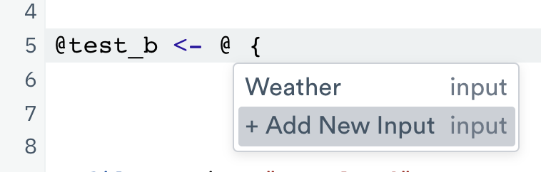
A subquery may use any dataset as an input by linking it. To do this, select + Add New Input from the Input menu in the OPAL console:

// Filter and extract from Observation
@test_a <- @Observation {
  filter (not if_null(EXTRA.poller_type)) and (string(EXTRA.poller_type) = "weather")
  make_col city:string(FIELDS.name)
  filter city="Chicago"
}

// Weather/Raw Events also has weather data
@test_b <- @WeatherRawEvents_41074100 {
  make_col city:string(FIELDS.name)
  filter city="Portland"
}

// Combine the two, extracting an additional field
@test_c <- @test_a {
  union @test_b
  make_col description:string(FIELDS.weather[0].description)
}

// Add another filter to the final result
<- @test_c {
  filter contains(description, "cloud")
}
}

Additional OPAL syntax details

Comments

OPAL allows single line comments beginning with // anywhere whitespace is permitted, except inside a literal string. Ctrl+/ comments or uncomments selected lines in the OPAL console. For multi-line comments, you may also use /* and */ start and end delimiters.

// only need deviceId and label
make_col deviceId:string(FIELDS.deviceInfo.deviceId), label:string(FIELDS.deviceInfo.label)

/*
 * TODO: better handle null deviceID values
 */

filter not if_null(deviceId) // ignore anything without a deviceId
}

Multi-line statements

Indent to continue a statement on the next line:

// select only the needed fields
pick_col
  time,
  deviceId:string(fields.deviceEvent.deviceId),
  sensor:string(fields.deviceEvent.attribute),
  value:float64(fields.deviceEvent.value),
}

Also, regular expressions may be broken into smaller units on multiple lines. Note that each component of a larger regex must be a valid regex, and are whitespace delimited:

// these two statements are equivalent
extract_regex data, /(?P<deviceid>[^|]*)|count:(?P<counts>[^|]*)|env:(?P<env>[^|]*)/

extract_regex data, /(?P<deviceid>[^|]*)|/
  /count:(?P<counts>[^|]*)|/
  /env:(?P<env>[^|]*)/
}

Field names

Most field (column) names may contain any character except the following:

• Double quote "
• Period .
• Backslash \
• Colon :
• Non-printable ASCII characters 0-31 (0x00-0x1F)

Field names may be up to 127 characters long, and Unicode and emoji are allowed. Names containing only alphanumeric (A-Z, a-z, 0-9) or underscore (_) characters may omit the double quotes.

make_col temperature:int64(field1)
make_col "count":int64(field2)
make_col "ΔT":float64(field3)
make_col "占用率":float64(field4)
make_col "0_3µm":float64(um03)
make_col "✅":bool(done)
}

To reference a field with non-alphanumeric characters, use double quotes and prepend @..

make_col temp_difference:@."ΔT"
}

📘

Note

Regex extracted columns from extract_regex are limited to alphanumeric characters (A-Z, a-z, 0-9).

Case-sensitivity

OPAL is case sensitive by default. When you reference or search Observe objects and column names, case is required to match.

There are a few local options for case insensitivity:

• Non-quoted search terms always match case-insensitively (though quoted search terms are case sensitive). See OPAL examples.
• The match_regex function can use regular expression engine flags to be case-insensitive. See match_regex.
• The filter verb can use syntax cues to be case-insensitive.

Using Links

Linking fields to Resources is a valuable and useful way to use Observe's features. Linked fields are green in the data grid, and have special context menus and click behavior. Note that referencing these fields in OPAL requires extra syntax. For instance, you may have a link named Session from a session_id column to a Sessions resource dataset. Referring to Session in OPAL will produce an error because that column is not actually in this data. Instead, you can use label(^Session) to refer to this column. The OPAL editor will automatically offer this construction when you type Session, so in most cases you will only need to allow it to replace your entry.

Using tags

Correlation tags provide a flexible way to link and correlate data across datasets in Observe. Tags are referenced in OPAL using the # symbol followed by the tag name. They can be used in filters and other OPAL operations just like regular columns. The OPAL editor provides autocomplete suggestions for available tags in your dataset, displaying them with the # prefix.

// Using tags in comparisons
filter #k8s.deployment.name = "cart-service"

// Using a tag as a grouping condition
timechart 1h, count(), group_by(#k8s.container.name)

📘

Note

Tags cannot be used in join conditions. Use regular columns or links for joining datasets.

Tag names may contain alphanumeric characters (A-Z, a-z, 0-9), underscores (_), and periods (.). For tag names with spaces or special characters, use quotes after the # symbol.

// Filter by a simple tag
filter #k8s.cluster.name = "prod-cluster"

// Filter by a tag with spaces or special characters
filter #'service name' = "auth-service"

For more information about correlation tags and how to add them to datasets, see Correlation tags.