Shape your data using stages
Follow this tutorial to understand using OPAL to shape your data using Stages.
Scenario
In this scenario, you have an Internet of things (IoT) system sending weather data in two formats. You want to manipulate the data and create a coherent picture of the weather.
In this tutorial, you learn how to manipulate your data using OPAL, the language used by Observe to perform database tasks.
Ingest data into Observe
Before working with OPAL, you must ingest your data into Observe using a Datastream and an Ingest Token. Use the following steps to start your ingestion process:
- Log into your Observe instance, and select Data & integrations > Datastreams from the left navigation.
- Click Create Datastream.
- Enter IntroductionToOPAL as the Name.
- (Optional) Enter a short description of the Datastream.
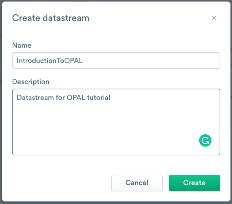
- Click Create.
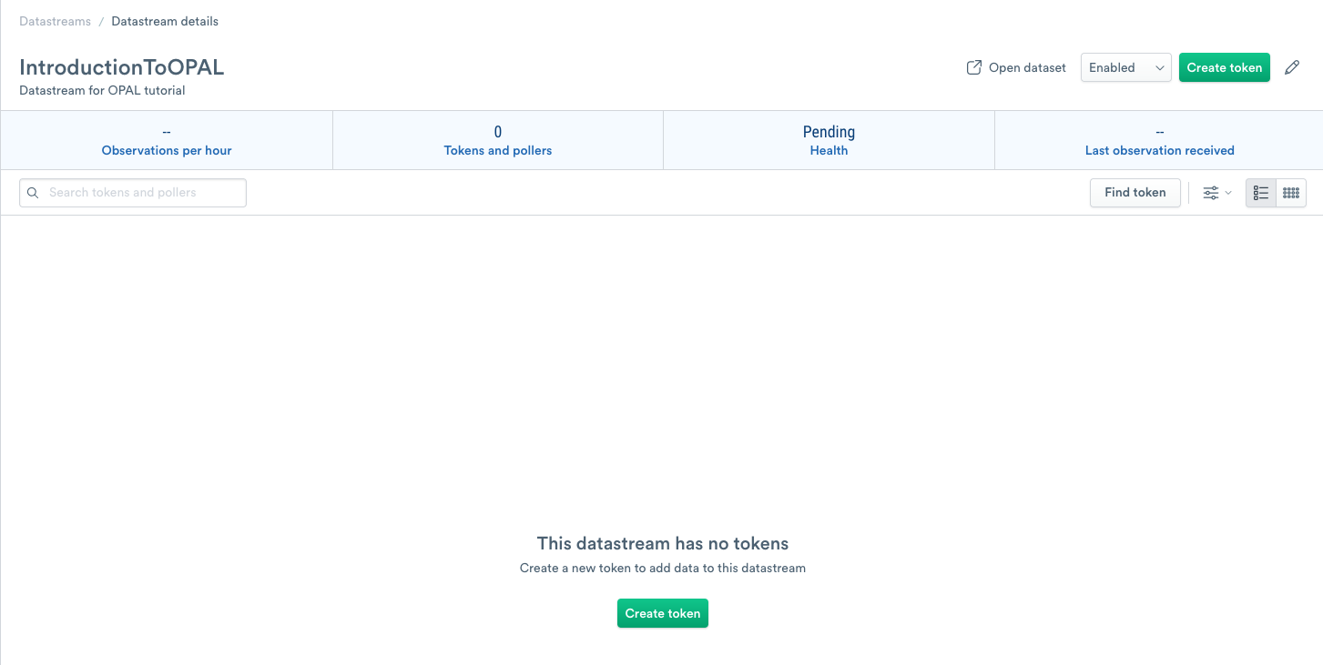
Add an ingest token to your datastream
To allow data into your Datastream, you must create a unique ingest token. Use the following steps to create an ingest token:
- To add a new ingest token, click Create token.
- Enter IntroductionToOPALToken as the name.
- (Optional) Enter a short description of the ingest token.
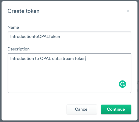
- Click Continue.
- You receive a confirmation message confirming the creation of your token creation and the token value.
- Click Copy to clipboard to copy the token value and then save it in a secure location.
NoteYou can only view the token once in the confirmation message. If you don’t copy and paste the token into a secure location, and you lose the token, you have to create a new one.
- Once you copy it into a secure location, select the confirmation checkbox, and then click Continue.
- After you click Continue, Observe displays setup instructions for using the new ingest token.
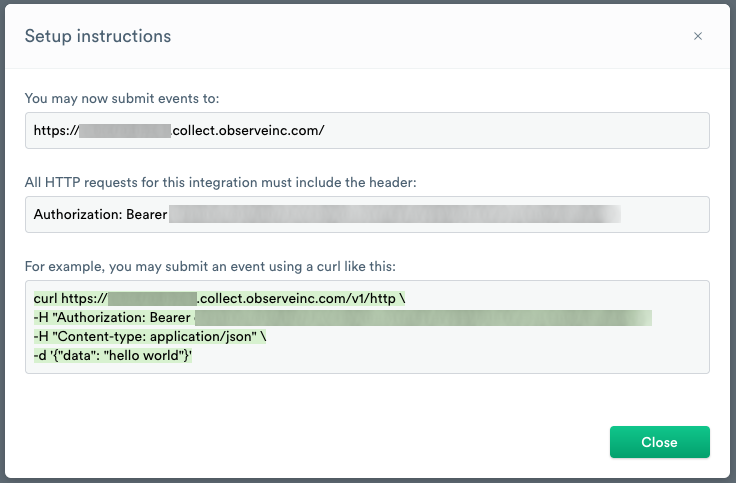
The URL https://{customerID}.collect.observeinc.com/ displays your customer ID and URL for ingesting data.
NoteSome Observe instances may optionally use a name instead of Customer ID; if this is the case for your instance, contact your Observe data engineer to discuss implementation. A stem name will work as is, but a DNS redirect name may require client configuration.
HTTP requests must include your customer ID and ingest token information.
You can view the setup instructions on your Datastream’s About tab.
Use cURL to ingest data into the tutorial datastream
This tutorial uses log files containing weather data that you must send to your Observe instance. Download both files from GitHub.
After you download the files, put them in the following locations:
- macOS -
home/<yourusername> - Windows -
C:\Users\<yourusername
You can send this data to the v1/http endpoint using cURL. See Endpoints for more details.
Details about the URL
You can encode the path component of the URL as a tag. To accomplish this, add the path, OPAL102, and the query parameter, format. Keep this information in mind for use later in the tutorial.
Copy and paste the following cURL to ingest the log data into the Datastream. Replace ${CustomerID} with your Customer ID, such as 123456789012. Replace{token_value} with the token you created earlier.
curl "https://${CustomerID}.collect.observeinc.com/v1/http/OPAL102?format=log" \
-H "Authorization: Bearer {token_value}" \
-H "Content-type: text/plain" \
--data-binary @./Measurements.MessyLog.log
curl "https://${CustomerID}.collect.observeinc.com/v1/http/OPAL102?format=jsonarray" \
-H "Authorization: Bearer {token_value}" \
-H "Content-type: application/json" \
--data-binary @./Measurements.ArrayOf.jsonEach cURL command returns {"ok":true} when successful.
After ingesting the data, you should see the data in the Datastream, OPAL102Token.
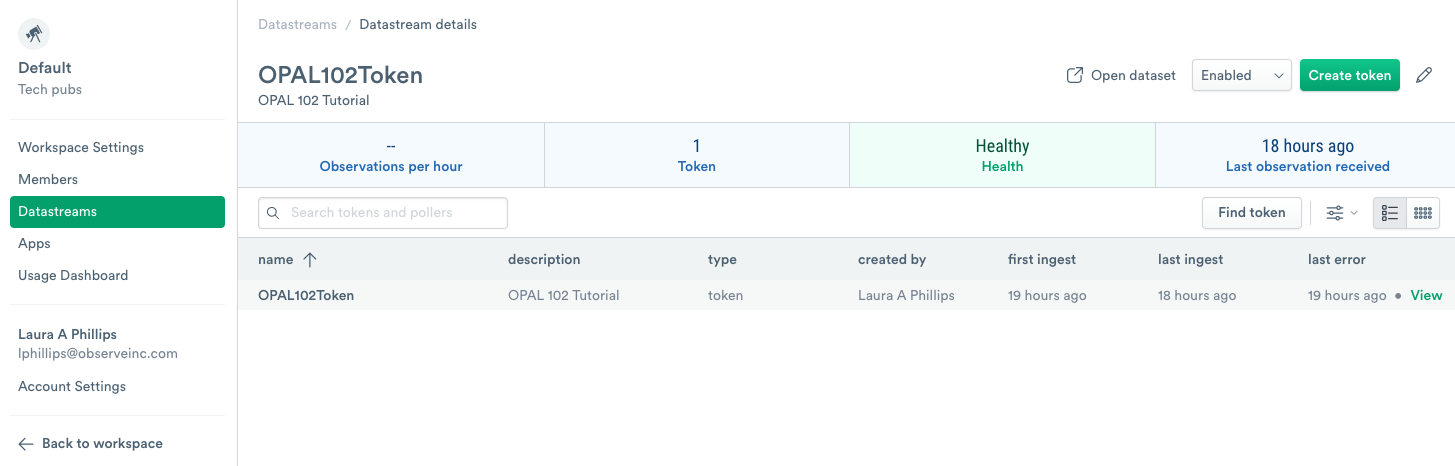
- Click Open dataset to view the ingested data.
- Select a row to display more information about that log event.
Create stages and configuration plan
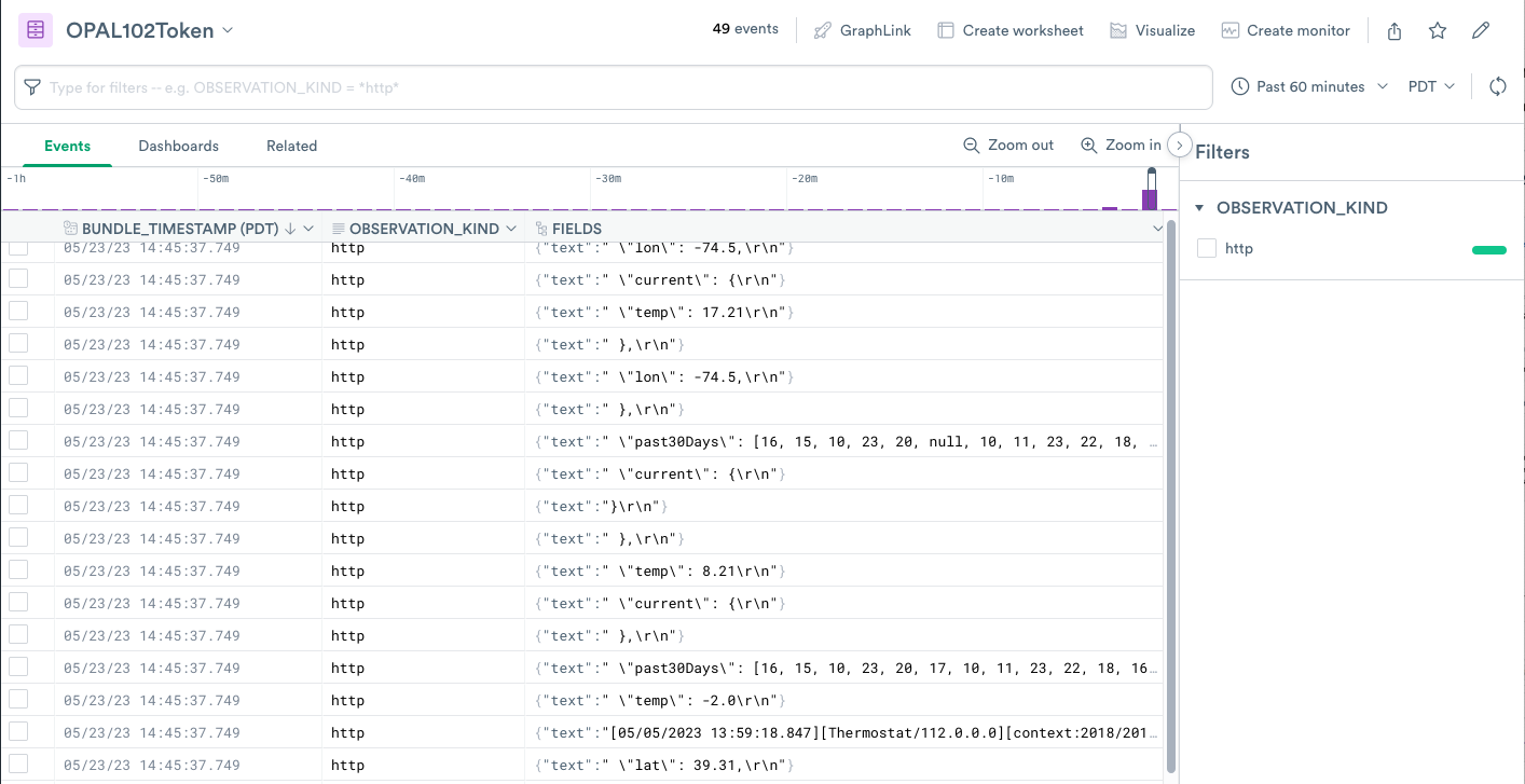
In this exercise, you have an IoT system sending weather data. The system sends data in two formats:
Measurements.ArrayOf.jsonfile sent in anapplication/jsonformat, where each semi-structured chunk of data automatically treated by Observe as a complete observation.Measurements.MessyLog.logfile sent astext/plainformat, with some unstructured data and some semi-structured data on multiple lines. Observe treats each line of the file as a separate observation. Log tracing systems send this data format because it has no knowledge about the type of message.
When you ingest the files, Observe stores them in the Observe DataStream. You can manipulate different types of messages and normalize them into a coherent whole using a concept called stages. A stage consists of an individual results table in a Worksheet. Stages can be linked and chained together in sequences and branching.
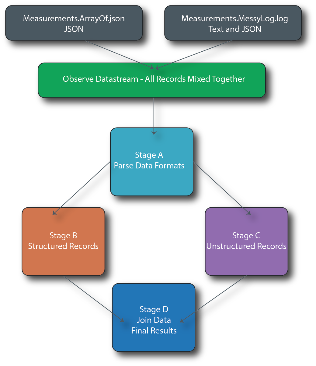
Hierarchy and graph for building stages
In this scenario, you perform the following tasks:
- Create Stage A - All Records by Type to decide the incoming format from the Datastream.
- Create Stage B - Structured Records derived from Stage A to convert unstructured datasets from
Measurements.MessyLog.loginto structured data. - Create a Stage C - Unstructured Records derived from Stage A to turn structured datasets from
Measurements.ArrayOf.jsonand perform light processing to match the structure from Stage B. - Join data from Stage B and Stage C together in Stage D - Structured And Unstructured Records and perform the additional processing and formatting on the joined data.
Create stage A - all records by type
Perform the following tasks:
- To create a Worksheet and start modeling your data, click Create Worksheet at the top of your OPAL102Token Dataset.
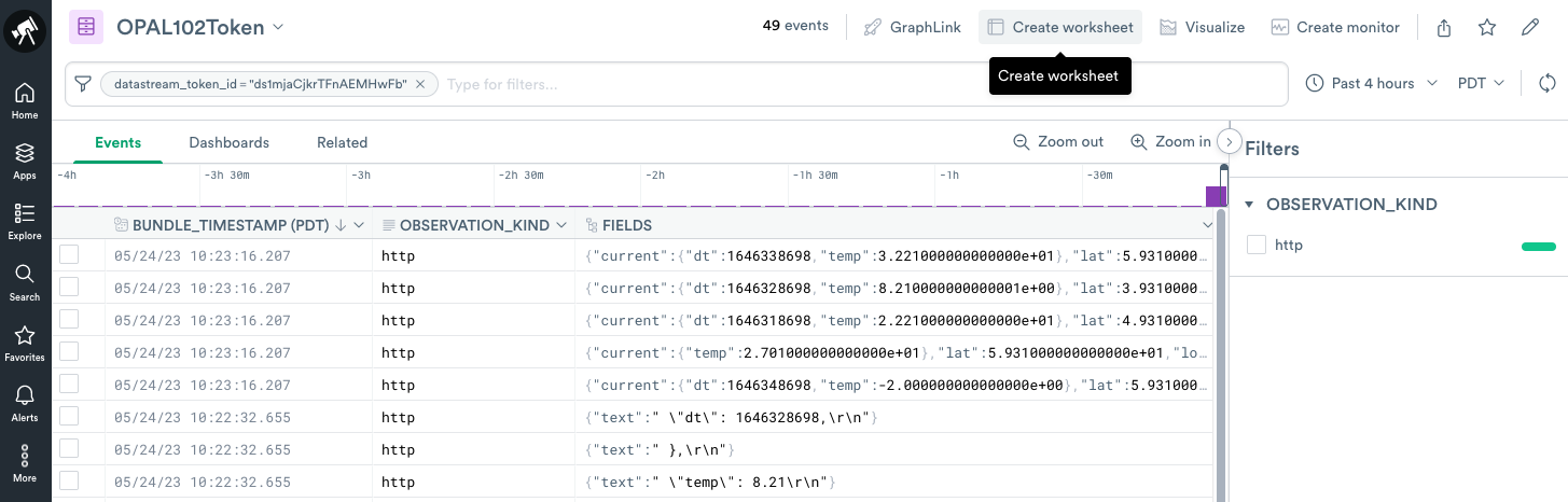
- Rename the name of the only stage in the worksheet from Stage 1 to Stage A - All Records By Type.
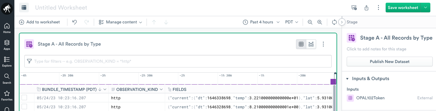
- Add the following OPAL code in the OPAL console:
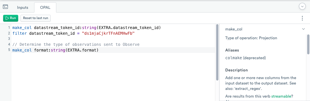
Classify records using the filter function
filter functionCreate a format column containing either jsonarray or log values based on parameters of the query string of cURL requests that sent the data to Observe.
You can review this type of extraction from raw observations and filtering in the Get started with OPAL tutorial.
Create stage B - structured records
Perform the following tasks:
- Add a second stage that builds on the previous Stage A by clicking Link New Stage at the bottom of the Worksheet.
- Rename the stage to Stage B - Structured Records.
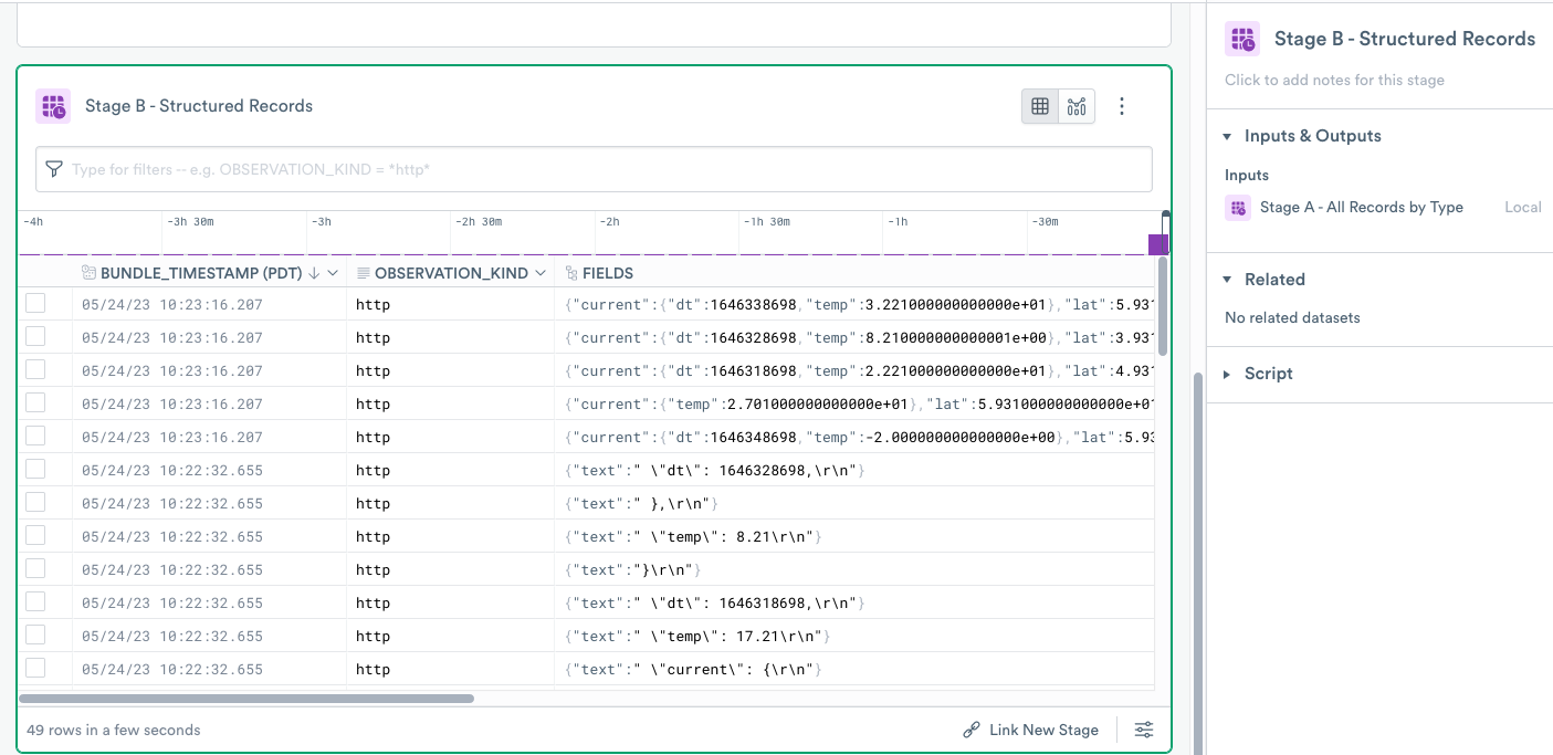
- Add the following OPAL code to your OPAL console:
Step 1 - use filter to filter data
filter to filter dataIn the following OPAL code, the filter function filters the data to only records containing the jsonarray value in the format column:
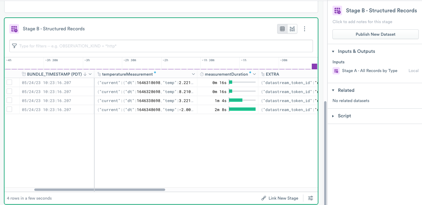
Step 2 - use rename_col to rename an existing column
rename_col to rename an existing columnStep 2 renames the existing column using the rename_col function. These records ingested into Observe with the application/json format, and automatically stored in the FIELDS column in any data type. This datatype is ready to be used.
Use the rename_col projection operation to simply rename the FIELDS column to temperatureMeasurement. Not creating a new column saves processing resources in the data conversion pipeline.
Step 3 - use path_exists to check for key existence
path_exists to check for key existenceIn this example, one of the measurements does not contain the current.dt key, and for purposes of this tutorial, considered invalid. This OPAL code in Step 3 uses the path_exists function to test for the existence of this key.
Example of a valid measurement:
{
"measurementDur": 128,
"lat": 59.31,
"lon": -64.5,
"current": {
  "dt": 1646348698,
  "temp": -2.0
}
"past30Days": [10, …]
}
{
"measurementDur": 256,
"lat": 59.31,
"lon": -64.5,
"current": {
"temp": 27.01 },
"past30Days": [16, …]
}Step 4 - use duration_sec to convert a numeric value to a duration
duration_sec to convert a numeric value to a durationStep 4 converts numeric values, measurementDur, to durations using the duration_sec function:
Create stage C - unstructured records
Perform the following tasks:
- Return to Stage A and click Link New Stage to add a third stage.
- Rename the new stage to Stage C - Unstructured Records.
Add the following block of OPAL code and click Run:
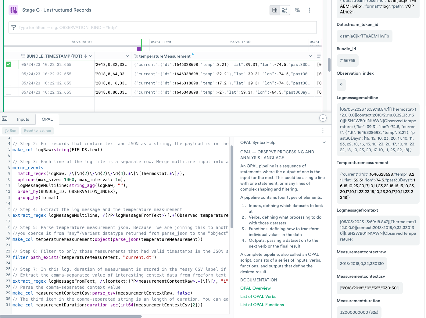
Step 1 - use filter to filter the data
filter to filter the dataThis step filters data from Stage A to contain only records with the value log in the format column. Focusing only on the desired records saves processing resources.
Observe ingests these records in the text/plain format and automatically stores them in the FIELDS column as an object of any data type with each incoming line in a text key, for example,
{"text":"[05/05/2023 13:59:18.847][Thermostat/112.0.0.0][context:2018/2018,0,64,330130][I:SH2WB01IN1AWN]Observed temperature: {\r\n"}
{"text":"    \"lon\": -74.5,\r\n"}
{"text":"[05/05/2023 13:59:18.847][Thermostat/112.0.0.0][context:2018/2018,0,32,330130][I:SH2WB01IN1AWN]Observed temperature: {\r\n"}
{"text":"        \"dt\": 1646338698,\r\n"}
{"text":"        \"dt\": 1646318698,\r\n"}
{"text":"    \"lat\": 39.31,\r\n"}
{"text":"    \"current\": {\r\n"}
Step 2 - use make_col to project a new column
make_col to project a new columnEach row contains a single observation, but Observe can merge the related items into a single value. Use the make_col projection operation to extract the FIELDS.text key and cast the value to logRaw string column. This allows you to prepare to merge events in the next step.
Step 3 - use merge_events to combine events
merge_events to combine eventsEach line of the log file is a separate row. Merge multi-line input into a single logical event.
Use the merge_events aggregate verb to merge consecutive events into a single event.
Details about each OPAL statement:
To match the first row for merge_events, use match_regex function to find the row that begins the event.
The options function is a special function to provide options to modify the behavior of various functions. It takes key/value pairs of modifiers. For the merge_events function, use max_size to indicate the maximum number of events to merge and max_interval and the maximum duration between the first and last event. For this tutorial, the selected value, 1 minute, could be too generous, but for real-world examples, it is possible to have some time skew between incoming records that should be merged. Larger match intervals can lead to using more computational credits used in processing data.
The string_agg aggregate function combines multiple values separated by a delimiter.
The order_by clause forces the right sequence of events to be combined. The default time order for order_by is time-ascending. When records are ingested using the cURL command, all of the timestamps for those records are within nanoseconds of each other, and all file contents have the same BUNDLE_ID. Each line has a unique, increasing OBSERVATION_INDEX, making it easy to reconstruct the order of lines.
If you don't specify group_by, the default grouping for merge_events becomes a set of primary key columns. In this example, you have not defined any primary keys and for completeness, use the format column, which in this stage is always the same.
Step 4 - use extract_regex to split unstructured and structured data from a string
extract_regex to split unstructured and structured data from a stringExtract the log message and the temperature measurement using the following OPAL code.
You reconstructed multiple lines of ingested log files into a single event in logMessageMultiline string column, and in this section, use the extract_regex verb to convert unstructured strings into structured data. This produces the logMessageFromText and the temperatureMeasurement string columns with the latter one containing a JSON string to parse.
Step 5 - use parse_json and object to create an object from a JSON string
parse_json and object to create an object from a JSON stringParse the temperature measurement JSON. Because you joined this to another column of object datatype, extract it from the "any"/variant datatype returned from parse_json to the object datatype.
OPAL Details
make_col temperatureMeasurement:object(parse_json(temperatureMeasurement))
//       ^^^^^^^^^^^^^^^^^^^^^^                                            New column name
//                              ^^^^^^                                     casting of 'any' type variable to 'object' type variable
//                                    ^^^^^^^^^^^                          parsing of json from text
//                                                ^^^^^^^^^^^^^^^^^^^^^^   text value to parse
The parse_json function parses the string into a temperatureMeasurement column of any data type which can be an object or an array data type. In a later stage when you combine this Stage C - Unstructured Records with results of Stage B - Structured Records, the types of columns must match, and the temperatureMeasurement column in Stage B - Structured Records is already an object data type. Therefore, use the object function to coerce this column to the object data type.
Step 6 - use path_exists to check for key existence in object data
path_exists to check for key existence in object dataThis step uses the same logic as Step 3 of Create stage B - structured records.
Step 7 - use parse_csv to parse CSV strings
parse_csv to parse CSV stringsIn this log, the duration of the measurement is stored in the messy CSV label and you extract the comma-separated value of interesting context data from free-form text.
OPAL Details
// Extract the comma-separated value of interesting context data from freeform text
extract_regex logMessageFromText, /\[context:(?P<measurementContextRaw>.*)\]\[/, "i"
//                                               ^^^^^^^^^^^^^^^^^^^^^^
// Parse the comma-separated context value
make_col measurementContextCsv:parse_csv(measurementContextRaw)
//                             ^^^^^^^^^
//                                       ^^^^^^^^^^^^^^^^^^^^^
// The third item in the comma-separated string is the length of duration.
make_col measurementDuration:duration_sec(int64(measurementContextCsv[2]))
// ^^^^^^^^^^^^ | OPAL | Description |
|---|---|
measurementContextRaw | The column you want to extract with the regular expression. |
parse_csv | Parse the CSV value. |
measurementContextRaw | The column to parse the CSV from. |
duration_sec | Convert the value of the duration to seconds. |
The example log message, when stripped of the JSON, contains a context block with some values:
[05/05/2023 13:59:18.847][Thermostat/112.0.0.0][context:2018/2018,0,16,330130][I:SH2WB01IN1AWN]Observed temperature:
                                                ^^^^^^^^^^^^^^^^^^^^^^^^^^^^^ you want this value
In this message, you extract the comma-separated string with the extract_regex function, and use the parse_csv function to convert it into an array.
The third item in the comma-separated string is the duration length. You can index it for display purposes.
The third value of the array, arrays in OPAL are 0 based, so index 2, contains the duration of the measurement taken by the sensor which you change to duration data type using the duration_sec function, just like in Step 4 of Create stage B - structured records.
Create stage D - structured and unstructured Records
You have split the processing of data from Stage A into Stage B and Stage C. Now you bring the processing of the data back into a single stage.
Add a stage that links to Stage B using the following steps:
- Return to Stage B.
- Click Link New Stage to add a fourth stage.
- Rename the new stage to Stage D - Structured and Unstructured Records.
- Click Input next to the OPAL console and then click Add Input.
- Select the Stage C - Unstructured Records stage.
When you add input to the Stage, Observe creates a reference to another Stage with a certain auto-generated suffix. If you named your Stages as presented in the tutorial, the name of Stage reference should be Stage C - Unstructured Records-tc62_. If not, then adjust your OPAL input accordingly.
Add the following block of OPAL code to the OPAL console:
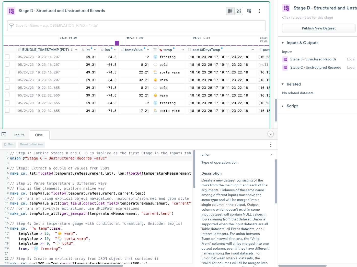
Step 1 - use union to combine the results of multiple stages
union to combine the results of multiple stagesUse the union verb to combine results of B - Structured Records and C - Unstructured Records stages.
If you named the stages as stated in each section, the name of the stage reference should be C - Unstructured Records_-tc62 because Observe adds a small semi-random hash to the name of the variable.
Unlike direct database engines where the unioned tables are often mandated to be identical, in Observe, the union verb does not require this. The two stages don’t fully match, and any records where columns are not shared receive NULL values in the opposite dataset.
Step 2 - use make_col and float64 to extract numeric values from a JSON object
make_col and float64 to extract numeric values from a JSON objectIn this step, you extract latitude and longitude from the JSON object representing the measurement of data. The object was reconstructed from multiple text lines in the Stage C - Unstructured Records and turned into an object, and parsed the same way as the object that arrived to Observe already in one piece.
Step 3 - use get_field or get_jmespath to extract numeric values from a JSON object naitvely
get_field or get_jmespath to extract numeric values from a JSON object naitvelyIn this step, you can see three ways of addressing JSON object paths using OPAL.
In the sample data, the observation has the following format:
{
    "measurementDur": 16,
    "lat": 49.31,
    "lon": -74.5,
    "current": {
        "dt": 1646318698,
        "temp": 22.21
    },
    "past30Days": [16, 15, ..., 18]
}
If you want to obtain the value of the temp key, a child of the current object, use OPAL with . (dot) notation and [0] indexers.
If you want to use explicit object navigation, OPAL uses a get_field function to extract a key from a given object. The function produces the same result as before, but uses more OPAL to do so.
//use explicit object navigation, newtonsoft/json.net and gson style
make_col tempValue_alt1:get_field(object(get_field(temperatureMeasurement, "current")), "temp")
//                      ^^^^^^^^^                                                        ^^^^ Get the 'temp' property of child object
//                                ^^^^^^
//                                       ^^^^^^^^^                          ^^^^^^^^          Get the 'current' property of parent object
//                                                 ^^^^^^^^^^^^^^^^^^^^^^                     Parent object
As a third option, OPAL implements a get_field function to use JMESPath, a query language for JSON. Unlike the previous two functions, get_field may be more expensive to use.
Step 4 - use case for conditional evaluation
case for conditional evaluationCreate a temperature gauge with conditional formatting and emojis.
Step 4 introduces conditional evaluation using the case function. OPAL evaluates conditions and results in pairs in the order of argument. The first successful evaluation to true ends execution.
This step also highlights that Observe platform allows for a bit of color and fun with any Unicode character, including emojis, in both the values and in field names.
NoteYou can use conditional formatting from the web interface to customize the presentation of your data.
Step 5 - use array, array_length, index_of_item, and slice_array to support arrays
array, array_length, index_of_item, and slice_array to support arraysLike all programming languages, OPAL supports arrays for creation, measurement, slicing, and indexing. Step 5 uses an array function to convert an implicit array from a JSON object to a real array, and an array_length function to measure the length of the array. The step also uses the index_of_item function to find an index of a specific item in the array, and the slice_array function to take the last 10 items from the longer array.
Step 6 - use pick_column to select the columns you want to display
pick_column to select the columns you want to displayYou’ve created a lot of intermediate columns so far in this tutorial. Now you can use the OPAL pick_col verb to choose the columns you want to see as the final result and optionally rename them.
Note to reference a field with non-alphanumeric characters like the fun emoji thermometer, you must use double quotes and prepend with @..
(Optional) Create stage E - ese one stage with Subqueries
A standard OPAL query consists of a linear series of steps with one or more dataset inputs. Using Stages as shown in this tutorial makes it possible to isolate portions of processing into logically isolated units of work and build data flows that split and merge as needed.
You can combine all the work you’ve done in earlier Stages into a single Stage with a single OPAL script. Observe enables this using the concept of Subquery . Logically, a Subquery is similar to a stage using an input Dataset.
A subquery consists of a name prefixed by the @ character followed by the definition in the curly brackets { with your OPAL inside}. You then invoke the subquery. In the following example, <- @ indicates the use of the default primary input, weather, without explicitly specifying it by name. The final <- @test_a {} invokes @test_a to generate the result:
Add a new stage
Perform the following steps to add a new stage:
- Select the OPAL102Token Event Dataset.
- Rename the stage to Stage E - Using just One Stage with Subqueries.
Add OPAL statements to the new stage
Add the following OPAL statements to the OPAL console, and click RUN.
Define the subqueries and interactions
Wrapping up the tutorial
To complete the tutorial, click the edit () icon in your Worksheet name your Worksheet OPAL 102 Building Structured and Unstructured Example. Click Save to save the Worksheet.
Summary of Key Topics in the OPAL 102 Tutorial
In this tutorial, you learned how to perform the following tasks:
- Create a Datastream to ingest data.
- Create an Ingest Token for the Datastream.
- Use cURL to ingest your log files into Observe in different formats.
- Create a Worksheet from your Dataset.
- Merge multiple events from multiple observation into single event.
- Use structured data to parse and manipulate JSON.
- Parse comma-separated values.
- Use array functions.
- Use type coercion.
- Use subqueries.
- Use Stages to split processing into logical chunks focused on just the applicable data.
- Use named subqueries to split processing.
Updated 6 months ago